In [1]:
%%sql
#count how many records are in my table
select count(*)
from [thematic-lore-110201:Natality_1980_1984.Births_1980_1984]
Out[1]:

In [2]:
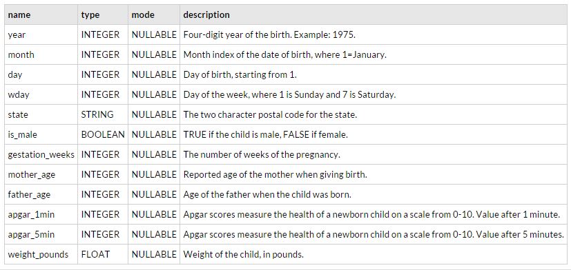
#check out the schema of the table
%bigquery schema --table thematic-lore-110201:Natality_1980_1984.Births_1980_1984
Out[2]:
bigquery command + pandas to make this sql into a dataframe
In [78]:
%%sql --module full_table
select * from [thematic-lore-110201:Natality_1980_1984.Births_1980_1984]
--it said the results were too large, so filtering down to one day
 where year = 1982 and month = 1 and day = 20
In [79]:
import gcp.bigquery as bq
import pandas as pd
In [80]:
df = bq.Query(full_table).to_dataframe()
len(df)
Out[80]:
Let's look at the data
In [11]:
df.head(10)
Out[11]:
In [55]:
#How many males and females born on this day?
groups = df.groupby('is_male')
groups.dtypes
for name, df_group in groups:
  if name == True:
    sex = 'male'
  else:
    sex = 'female'
  print '%d %s babies' % (len(df_group), sex)

#how many babies in each state?
groups = df.groupby(['state','is_male'])
table = pd.pivot_table(df, index='state', columns='is_male', aggfunc=len, values='year')
#create a column that is the total count by state, not split by group
table_totals = pd.pivot_table(df, index='state', aggfunc=len, values='year')
table = pd.concat((table,table_totals),axis=1)
#rename the columns
table.columns = ['female','male','total']
#display
groups.size()
table
Out[55]:
chart births by month and year - line chart
In [3]:
%%sql --module birthdata
select year, month, concat(string(month),"/",string(year)) as yearmonth, count(*) as births
from [thematic-lore-110201:Natality_1980_1984.Births_1980_1984]
group by year, month, yearmonth
order by year, month
In [4]:
#put result of query in a dataframe
df_ym = bq.Query(birthdata).to_dataframe()
In [34]:
import matplotlib.pyplot as plt
plt.style.use('ggplot')
plt.figure();
df_ym.plot(x='yearmonth',y='births');

Now we'll recreate the getstation weeks vs birth weight scatterplot
In [13]:
%%sql --module gestation_weight
select gestation_weeks, weight_pounds
from [thematic-lore-110201:Natality_1980_1984.Births_1980_1984]
where year = 1982 and month = 1 and day = 20
and gestation_weeks < 99 and gestation_weeks is not null and weight_pounds is not null
--forgot to bring in live baby variable, so using apgar as proxy
and apgar_1min is not null and apgar_1min < 99
In [77]:
import numpy as np
#put result of query in a dataframe
df_gw = bq.Query(gestation_weight).to_dataframe()
df_gw_numeric = df_gw[np.isreal(df_gw).any(axis=1)]
#df_gw.plot(kind='scatter', x='gestation_weeks', y='weight_pounds')
x=df_gw_numeric['gestation_weeks']
y=df_gw_numeric['weight_pounds']
m,b = np.polyfit(x, y, 1)
yline = m*x+b # regression line

df_gw_numeric = pd.concat((df_gw_numeric,yline),axis=1)
df_gw_numeric.columns = ['gestation_weeks','weight_pounds','fit_line']

plt.figure()
df_gw_numeric.plot('gestation_weeks','fit_line','line',zorder=0);
plt.scatter(df_gw_numeric['gestation_weeks'],df_gw_numeric['weight_pounds']);
plt.xlim(10,60)
plt.show()

hm, still not as high of an R^2 as I would have expected! (similar for linear) Lots of variation in the weight even at similar weeks.