Principles of Data Visualization for Exploratory Data Analysis [presentation – pdf]
Principles of Data Visualization for Exploratory Data Analysis [paper – [pdf]
Check out the references in both documents for some good resources. I’ll include some links in the post below, too. I had a lot more material from my research that I wanted to include and just didn’t have time to in a 15-minute presentation! The professor was happy about the topic I picked because she’s teaching a class on Data Visualization next semester, so I think that worked out in my favor :)
These two books by Stephen Few covered the very basics of visualization for human perception:
Show Me the Numbers: Designing Tables and Graphs to Enlighten
Now You See It: Simple Visualization Techniques for Quantitative Analysis
Blog posts about related topics:
Six Revisions: Gestalt Laws
eagereyes: Illustration vs Visualization
Detailed visualization of NBA shot selection
Publications and articles:
IEEE Transactions on Visualization and Computer Graphics
Toward a Perceptual Science of Multidimensional Data Visualization: Bertin and Beyond by Marc Green, Ph. D.
Scagnostics by Dang and Wilkinson
Generalized Plot Matrix (GPLOM) by Im, McGuffin, Leung
UpSet: Visualization of Intersecting Sets by Lex, Gehlenborg, Strobelt, et al.
…and there are more resources in the paper and presentation files! (and if you’re REALLY interested in this topic, post a comment and I will add even more links I have bookmarked)
I also did a project using some data from my day job related to university fundraising and major gift prospects, but unfortunately I can’t share that study here because I don’t have permission to do so. It included some cool visuals like bubble charts, and also an interesting analysis of movement through the prospect pipeline using Markov Chains. I learned a lot doing that one!
It was nice to end my final semester of grad school with two data-related projects! (Yes, I’m finally graduating! Masters of Systems Engineering! woo hoo!)
]]>So, here’s a bit about what I’ve been up to data-science-wise:
- I’m in a grad class called Stochastic Models and we’re learning about Markov Chains right now. Fascinating stuff! Here’s a cool site that visually shows some Markov Chain concepts.
- My other grad class is Intro to Systems Engineering. (Yeah, because of the courses offered online, I’m taking the intro class in my second-to-last semester!) We just did a neat project in that class that involved coming up with a strategy and participating in a baseball draft, so I’ll come back later and write about that in more detail.
- I’m almost at the end of Udacity’s Cloudera Hadoop course. I am really enjoying learning about MapReduce, and will definitely write up a review of the class when I’m done. The biggest frustrations I’ve had so far haven’t involved the Hadoop concepts, but using the VM they provide has been frustrating! All I have left on that is the final project, so soon i’ll be able to cross that one off my goals list.
- Soon, I need to come up with a final project for my Systems Engineering Masters degree. I’m definitely doing something data science related, and will update when that plan is finalized.
- I’ve been telling more people about my data science plans, and have had more people asking me about data science and the learning process. I may be giving a talk to my alma mater’s IEEE Computer Society club meeting soon about “What is data science?”, so that will be fun!
Are you “becoming a data scientist”, too? What projects are you in the middle of right now?
]]>Now I can cross that one off the list: Updated Goals
]]>Very good analysis and you showed great potential to become a good researcher!
Comments:
1. when you code your categories features, 1 of k coding is a good choice. Did you apply this method to all categories features?2. Some time, normorlize features will make a huge difference. One way to do this is to comput the z-score for features before you train a model on the data.
3. In terms of machine learning application, your analysis is good. If you try to find a social study expert to collobrate with you, I believe your findings can be published on high impacting journals.
4. In order to publish your work, you will need to do some research to found what have been done in this field.
This is especially encouraging since I want to become a data scientist, so hearing positive feedback like this, even encouraging me to publish after having only taken one semester of Machine Learning, feels great!
So, I will take time this summer to do more research and learning and expand on this project (since it was a rush to complete enough to turn in on time in this class but there’s a lot more I want to do with it), and I will collaborate with some people at the university where I work to further distill the results and see if we can apply them to segment out some potential first-time donors for next fiscal year.
This is fun!
]]>I settled on using SciKit-Learn (skLearn) Random Forest since I have been teaching myself Python throughout this class and kept seeing references to the skLearn package for machine learning. I like their site, and the documentation was good enough to get me started. skLearn also has tools for preprocessing data, which is something I knew I’d need since I was working with a “real world” data set, so I got started.
First, I decided on what problem to tackle. Since this was a classification project, I decided to see if I could identify people that gave to the university for the first time in a fiscal year, and compared “never givers” (non donors) to “first time donors”. I pulled data such as class year, record type (alumni, parent, etc.), college, zip code, distance from the school, whether we had an address/email/phone number for them, whether they were assigned to a development officer, how long their record had been in the database, how many solicitation and non-solicitation contacts they had with the university, whether they were a parent of a current student, had ever been an employee of the university, etc.
Many of these columns were yes/no (like Has Email) or continous (like distance), so didn’t need any modification except figuring out what to do when the field was null. I wrote functions to return values that I thought made sense for when the field was empty, and figured I’d play around with those a bit when I saw the results. I also tried excluding the rows with empty values in certain columns, but that made the result worse.
So, when I first ran the Random Forest (the code for this part was the easiest part of the project thanks to skLearn!), the scores looked like this:
Overall score: 98%
Class 0: 99%, 141,500 records
Class 1: 16%, 2,300 records
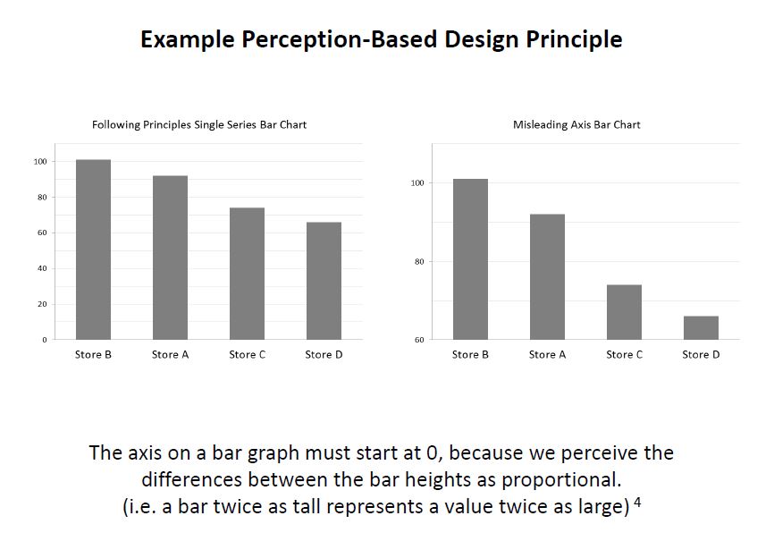
Class 0 had all of the records of everyone that had ever been added to our database for any reason but had not made a gift to the university, while class 1 consisted only of people who had made their first gift in Fiscal Year 2013. As you can see, I learned a lesson about working with an imbalanced dataset.
I learned how to output the “importances” of each column that the Random Forest used to classify the data and started manipulating my dataset. First, I tried “downsampling”, which means that you remove some records from the larger class so it doesn’t contribute so heavily to the results. I also brought in more fields that were categorical, such as the Record Type Codes, and used the skLearn Preprocessing functions “LabelEncoder”, which turned the string categories into numerical values, and “OneHotEncoder”, which then turned those numerical values into 1-of-k sparse arrays with the column value a 1 and every other value a 0. For instance, “AL” for Alumni would be category “1”, and encoded as [1 0 0 0 0 0 0 0 0] if there were 9 possible categories.
Eventually, I got the results to look like this:
Overall score: 99%
Class 0: 99%, 101,750 records
Class 1: 97%, 2,032 records
Now, there are some “wrong” reasons that I could have come out with such good results, so to better understand this (and to be able to use these results to provide any insight to the Office of Annual Giving), I need to figure out how to output the values that the Random Forest is using to classify each point (not just the weights of the columns). I am pretty sure there is a way to do this, but I just didn’t have time during this 2-week project which I mostly worked on late-night while working full time (luckily my manager gave me 2 days off during the final 2 weeks to work on this final project and another for my Risk Analysis class since they were each 30% of my grade). So, that will be my next step in learning how to better work with this type of data.
Additionally, I want to learn how to output some visualizations, such as a “scatter matrix” which plots each column in a dataset against every other column so you can visually spot which have strong correlations. (I plan to learn how to do that using this: Pandas Scatter Plot Matrix)
I also tried to see if my FY13 data could be used to predict FY14 first-time donors. There are some good reasons it wasn’t perfect, but it appears I was able to correctly classify 67% of the data points for first time donors, which I don’t think is too bad.
I have attached my project write-up and some python code if anyone wants to take a look. I can’t attach the dataset because of privacy and permission issues, but a sample row looks like this:
DATA_CATEGORY: FIRST TIME DONOR FY13
CLASSIFICATION: 1
FY14 RECORD TYPE: AL
YEARS_SINCE_GRADUATED: 2
PREF_SCHOOL_CODE: COB
OKTOMAIL: 1
OKTOEMAIL: 1
OKTOCALL: 1
EST_AGE: 24
ASSIGNED: 0
ZIP5: 23219
ZIP1: 2
MI_FROM_HBURG: 98.65
HAS_PREF_ADDRESS: 1
HAS_BUSINESS_ADDRESS: 0
HAS_PHONE: 0
HAS_EMAIL: 1
FY1213_SOLICIT_B4: 2
FY1213_NONSOLICIT_B4: 5
FY1213_SOL_NONOAG_B4: null
FY1213NONSOLNONOAGB4: 4
SOLICITATIONS: 2
NONSOLICITAPPEALS: 5
CURRENT_RECENT_PARENT: 0
EVER_EMPLOYEE: 0
YEARS_SINCE_ADDED: 1.00
YEARS_SINCE_MODIFIED: null
EVENT_PARTICIPATIONS: 0
Any feedback is welcome! I am very relieved that this semster is done, and I plan to spend the summer learning as much as possible about Data Science topics, so throw it all at me! :)
(Again, I have to change the .py file extensions to .txt for wordpress to allow me to upload)
607 ML Final Project Write-Up
So, to wrap up Project 3. I ended up getting the Neural Networks working in PyBrain, but when it came to Support Vector Machines (SVM), I just could not get it to run without errors. I had already downgraded to Python 2.7 to get PyBrain working at all, but there were further dependencies for the SVM functionality, and at midnight the night before it was due, I still hadn’t gotten it to run, so I figured it was time to try another approach. This is when I started looking at SciKit-Learn SVM.
I had wanted to do the whole project in PyBrain if possible, but it turned out that switching to SciKit-Learn (also called sklearn) was a good idea, because the documentation was helpful and the implementation painless. I had to tweak how I was importing the data from the training and test files since I was no longer using PyBrain’s ClassificationDataSet, but that wasn’t a complicated edit.
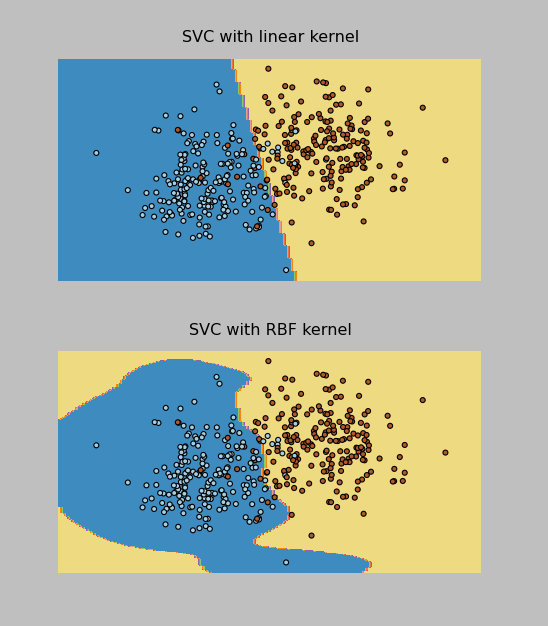
I was able to implement both the RBF and Linear kernel versions of the SVM Classifier (called SVC in sklearn). The Linear one actually worked better on the test data provided by the professor, and it correctly classified 96% of the data points (which were evenly split into 2 classes). In addition, I was able to make these cool plots by following the instructions here.
I have pasted the SVM code below and attached all of my project files to this post. Now on to the Final Project, due May 9.
Thanks to everyone that gave me tips on Twitter while I was working through the installations on this one!
import pylab as pl
import numpy as np
from sklearn import svm, datasets

print("\nImporting training data...")
#bring in data from training file
f = open("classification.tra")
inp = []
tar = []
for line in f.readlines():
    inp.append(list(map(float, line.split()))[0:2])
    tar.append(int(list(map(float, line.split()))[2])-1)


print("Training rows: %d " %  len(inp) )
print("Input dimensions: %d, output dimensions: %d" % ( len(inp), len(tar)))
#raw_input("Press Enter to view training data...")
#print(traindata)
print("\nFirst sample: ", inp[0], tar[0])

#sk-learn SVM
svm_model = svm.SVC(kernel='linear')
svm_model.fit(inp,tar)

#show predictions
out = svm_model.predict(inp)
#print(test)
class_predict = [0.0 for i in range(len(out))]
predict_correct = []
pred_corr_class1 = []
pred_corr_class2 = []
for index, row in enumerate(out):
    if row == 0:
        class_predict[index] = 0
    else:
        class_predict[index] = 1
for N in range(len(class_predict)):
    if class_predict[N] == tar[N]:
        if tar[N] == 0:
            pred_corr_class2.append(1)
        if tar[N] == 1:
            pred_corr_class1.append(1)
        predict_correct.append(1)
    else:
        if tar[N] == 0:
            pred_corr_class2.append(0)
        if tar[N] == 1:
            pred_corr_class1.append(0)
        predict_correct.append(0)

print ("SVM Kernel: ", svm_model.kernel)
print ("\nCorrectly classified: %d, Percent: %f, Error: %f" % (sum(predict_correct),sum(predict_correct)/float(len(predict_correct)),1-sum(predict_correct)/float(len(predict_correct))))
print ("Class 1 correct: %d, Percent: %f, Error: %f" % (sum(pred_corr_class1),sum(pred_corr_class1)/float(len(pred_corr_class1)),1-sum(pred_corr_class1)/float(len(pred_corr_class1))))
print ("Class 2 correct: %d, Percent: %f, Error: %f" % (sum(pred_corr_class2),sum(pred_corr_class2)/float(len(pred_corr_class2)),1-sum(pred_corr_class2)/float(len(pred_corr_class2))))


raw_input("\nPress Enter to start testing...")

print("\nImporting testing data...")
#bring in data from testing file
f = open("classification.tst")
inp_tst = []
tar_tst = []
for line in f.readlines():
    inp_tst.append(list(map(float, line.split()))[0:2])
    tar_tst.append(int(list(map(float, line.split()))[2])-1)


print("Testing rows: %d " %  len(inp_tst) )
print("Input dimensions: %d, output dimensions: %d" % ( len(inp_tst), len(tar_tst)))
print("\nFirst sample: ", inp_tst[0], tar_tst[0])

print("\nTesting...")

#show predictions
out_tst = svm_model.predict(inp_tst)
#print(test)
class_predict = [0.0 for i in range(len(out_tst))]
predict_correct = []
pred_corr_class1 = []
pred_corr_class2 = []
for index, row in enumerate(out_tst):
    if row == 0:
        class_predict[index] = 0
    else:
        class_predict[index] = 1
for N in range(len(class_predict)):
    if class_predict[N] == tar_tst[N]:
        if tar_tst[N] == 0:
            pred_corr_class2.append(1)
        if tar_tst[N] == 1:
            pred_corr_class1.append(1)
        predict_correct.append(1)
    else:
        if tar_tst[N] == 0:
            pred_corr_class2.append(0)
        if tar_tst[N] == 1:
            pred_corr_class1.append(0)
        predict_correct.append(0)

print ("\nTest Data Correctly classified: %d, Percent: %f, Error: %f" % (sum(predict_correct),sum(predict_correct)/float(len(predict_correct)),1-sum(predict_correct)/float(len(predict_correct))))
print ("Class 1 correct: %d, Percent: %f, Error: %f" % (sum(pred_corr_class1),sum(pred_corr_class1)/float(len(pred_corr_class1)),1-sum(pred_corr_class1)/float(len(pred_corr_class1))))
print ("Class 2 correct: %d, Percent: %f, Error: %f" % (sum(pred_corr_class2),sum(pred_corr_class2)/float(len(pred_corr_class2)),1-sum(pred_corr_class2)/float(len(pred_corr_class2))))
(I had to change the .py files to .txt in order for WordPress to upload them. The “zips” files are for the data sets that had 16 inputs and 10 classes.)
PyBrain_NeuralNet
PyBrain_NNClassification_zips
PyBrain_NNClassification2
SciKitLearn_SVM
SciKitLearn_SVM_zips
Here’s the output!
Importing training data...
Training rows: 3000
Input dimensions: 16, output dimensions: 1
('\nFirst sample: ', array([  1.       ,   1.       ,   1.       ,   0.       ,   0.       ,
         1.       ,   0.       ,   1.       ,  17.       ,   0.       ,
         0.4516129,   0.       ,   0.7931035,   0.902439 ,   0.8125   ,
         1.12037  ]), array([1, 0, 0, 0, 0, 0, 0, 0, 0, 0]), array([0]))

Creating Neural Network:
Network Structure:
('\nInput: ', <LinearLayer 'in'>)
('Hidden layer 1: ', <SigmoidLayer 'hidden0'>, ', Neurons: ', 13)
('Output: ', <SoftmaxLayer 'out'>)

Training the neural network...
train-errors: [  0.038761  0.029293  0.024884  0.022043  0.020121  0.018677  0.017529  0.016579  0.015792  0.014626  0.013603  0.012940  0.012482  0.012046  0.011884  0.011578  0.011182  0.011038  0.010635  0.010769  0.010317  0.010112  0.010432  0.009864  0.009588  0.009404  0.009336  0.009192  0.009064  0.008943  0.008755  0.009031  0.008283  0.008543  0.008208  0.008102  0.007873  0.007997  0.007970  0.007687  0.007473  0.007419  0.007206  0.007246  0.007052  0.006973  0.007284  0.007343  0.006806  0.007144  0.006771  0.006940  0.006789  0.006612  0.007002  0.006759  0.006553  0.006608  0.006518  0.006929  0.006351  0.006677  0.006509  0.006343  0.006221  0.006090  0.006272  0.006752  0.006091  0.006285  0.006146  0.006198  0.006449  0.006274  0.006259  0.006845  0.006471  0.006018  0.005944  0.005972  0.006273  0.006480  0.005726  0.006301  0.006516  0.006499  0.006223  0.006136  0.005867  0.005885  0.005876  0.005842  0.006032  0.005826  0.005653  0.005705  0.006175  0.005797  0.005788  0.005845  0.005603  0.004935]
valid-errors: [  0.063600  0.032400  0.026321  0.023301  0.021404  0.020292  0.018790  0.017495  0.016995  0.015580  0.014692  0.013846  0.014473  0.012946  0.012400  0.013170  0.012202  0.011508  0.011371  0.011360  0.011115  0.010672  0.011536  0.010711  0.010432  0.011160  0.010278  0.010163  0.010221  0.010590  0.009836  0.009849  0.009846  0.010072  0.009938  0.009178  0.008529  0.010189  0.008046  0.008211  0.009385  0.008088  0.008553  0.009059  0.007765  0.008596  0.008465  0.009120  0.008196  0.009056  0.008426  0.007434  0.007872  0.008579  0.009457  0.008823  0.007650  0.007414  0.008214  0.007400  0.007275  0.007797  0.008120  0.007587  0.008690  0.008652  0.007537  0.008202  0.007392  0.008514  0.007407  0.007521  0.007788  0.007296  0.007375  0.007785  0.008493  0.009074  0.007640  0.007837  0.007370  0.009581  0.007429  0.007780  0.007485  0.008100  0.007646  0.008031  0.007486  0.009158  0.007781  0.007797  0.007320  0.007511  0.008301  0.008997  0.007239  0.007497  0.008476  0.007089  0.008157  0.006774]


<FullConnection 'FullConnection-4': 'hidden0' -> 'out'>
(0, 0) 1.97034676195
(1, 0) 0.205547544009
(2, 0) -1.39194384331
(3, 0) -1.19536809665
(4, 0) 0.532497209596
(5, 0) 3.78538106374
(6, 0) 2.96117412924
(7, 0) -3.78523581656
(8, 0) -2.33305927664
(9, 0) -0.107099673461
(10, 0) 1.05253692747
(11, 0) 1.16998764128
(12, 0) -1.6446456627
(0, 1) -3.78554660125
(1, 1) 0.110082157195
(2, 1) 2.00959920575
(3, 1) -1.4818647156
(4, 1) 0.47754811455
(5, 1) 0.586612033935
(6, 1) -3.33060359627
(7, 1) 3.47983943215
(8, 1) 0.68663692996
(9, 1) -1.33694729559
(10, 1) 1.41119329168
(11, 1) -0.808565967083
(12, 1) 2.36545357056
(0, 2) 2.0686653235
(1, 2) -0.928835048313
(2, 2) 1.83676782784
(3, 2) -1.76161763582
(4, 2) 0.9361187835
(5, 2) -5.18245128877
(6, 2) 0.716382960297
(7, 2) -3.60545617741
(8, 2) -0.402315012393
(9, 2) -1.58503008135
(10, 2) 2.83977738833
(11, 2) 0.785279233021
(12, 2) -1.18054754169
(0, 3) -0.203951751624
(1, 3) 0.322602700012
(2, 3) -0.135262966169
(3, 3) -1.41762708896
(4, 3) -4.84104938707
(5, 3) -1.25393926994
(6, 3) 2.17559963467
(7, 3) -2.09770282748
(8, 3) 0.616624009402
(9, 3) 2.02261312669
(10, 3) 2.50046686569
(11, 3) 1.21013636278
(12, 3) -2.02479566929
(0, 4) 0.262402966139
(1, 4) -0.2049562553
(2, 4) 1.46174549966
(3, 4) 5.80019891011
(4, 4) -0.977813743463
(5, 4) 0.866255330743
(6, 4) -0.623536140065
(7, 4) 2.31791322416
(8, 4) 2.45985579544
(9, 4) -0.773406462405
(10, 4) -3.01271325372
(11, 4) -0.394620653754
(12, 4) -2.51727744427
(0, 5) -1.84884535137
(1, 5) 4.12641600292
(2, 5) -1.71652533043
(3, 5) -0.0815174955082
(4, 5) -0.293698800606
(5, 5) 1.71536468963
(6, 5) -0.09204101225
(7, 5) -3.39683666138
(8, 5) 2.65257065343
(9, 5) 1.24530888054
(10, 5) -1.03146066497
(11, 5) -1.21429970585
(12, 5) 0.729863849101
(0, 6) 2.04586824381
(1, 6) 0.49739573113
(2, 6) 2.57776903746
(3, 6) -1.93553170732
(4, 6) 2.78487687106
(5, 6) 1.3000471899
(6, 6) -4.73027055616
(7, 6) -2.46351648945
(8, 6) -0.28859559781
(9, 6) -2.02233867248
(10, 6) -0.156622792383
(11, 6) 1.92189313946
(12, 6) -2.23854617011
(0, 7) -2.24824282938
(1, 7) -0.980973854304
(2, 7) -4.37502761199
(3, 7) -0.480980045708
(4, 7) 1.27159949426
(5, 7) -3.34473044103
(6, 7) 1.40822677342
(7, 7) 4.47168119792
(8, 7) 0.344224226657
(9, 7) -0.507463253978
(10, 7) 3.00263456183
(11, 7) 1.41026234082
(12, 7) -1.63287505494
(0, 8) 1.85402453493
(1, 8) -0.655788582737
(2, 8) -0.725833018627
(3, 8) -0.422927874452
(4, 8) 3.01031150439
(5, 8) -0.11160243227
(6, 8) -0.945132529229
(7, 8) -1.7545689227
(8, 8) -1.21431898252
(9, 8) 2.22819018763
(10, 8) 0.260729007609
(11, 8) -2.52922250574
(12, 8) -0.56668568841
(0, 9) 0.0364945847699
(1, 9) -0.237982860432
(2, 9) -2.62646677443
(3, 9) 1.0732844588
(4, 9) -0.259593431419
(5, 9) -0.848517900957
(6, 9) 2.508395978
(7, 9) 3.30027859271
(8, 9) 0.403155991036
(9, 9) 2.80187580798
(10, 9) 0.482560709585
(11, 9) -0.667975028034
(12, 9) 0.900458124988
<FullConnection 'FullConnection-5': 'in' -> 'hidden0'>
(0, 0) 3.08811266325
(1, 0) -0.349496643363
(2, 0) 1.30386752112
(3, 0) -1.98774338878
(4, 0) -1.32967911522
(5, 0) 1.08797500734
(6, 0) -0.0471055794106
(7, 0) -0.869646403657
(8, 0) 1.75310037828
(9, 0) 1.68139639596
(10, 0) 0.338577992907
(11, 0) -0.893166683793
(12, 0) -0.221695458268
(13, 0) -0.973468822585
(14, 0) -2.35309393784
(15, 0) -0.215912101451
(0, 1) -4.17148121547
(1, 1) 2.51239249638
(2, 1) -2.3835748258
(3, 1) -0.921878525015
(4, 1) 0.00582746958346
(5, 1) -0.382111955259
(6, 1) 0.753175222035
(7, 1) 1.25959664026
(8, 1) -0.683135069059
(9, 1) -0.209658642682
(10, 1) 0.218220380222
(11, 1) -0.0446428066644
(12, 1) -0.0416074753453
(13, 1) -0.91371785665
(14, 1) -0.632054483002
(15, 1) 1.57790399324
(0, 2) 3.62327710485
(1, 2) -3.27317649121
(2, 2) -0.839175648632
(3, 2) 0.412688954247
(4, 2) 2.44336416739
(5, 2) 1.21796013909
(6, 2) 3.1687123603
(7, 2) 0.948876278654
(8, 2) -0.286973680858
(9, 2) -1.9075156445
(10, 2) -1.14925901374
(11, 2) -0.0210168332583
(12, 2) -0.0909940901091
(13, 2) -2.61880332586
(14, 2) -0.437724207854
(15, 2) 1.20185096351
(0, 3) -1.02510071023
(1, 3) -1.02697812149
(2, 3) -1.63897260494
(3, 3) 3.11149300751
(4, 3) -1.04298253508
(5, 3) 1.96548080077
(6, 3) -2.27063951013
(7, 3) 0.96011424472
(8, 3) 0.0164849529198
(9, 3) -0.253354500755
(10, 3) -2.28882965008
(11, 3) -0.283636888249
(12, 3) -1.99865996877
(13, 3) 1.52667642474
(14, 3) -0.0228903198235
(15, 3) 0.0135050503295
(0, 4) -2.14139223479
(1, 4) -2.8408497749
(2, 4) 3.81399104479
(3, 4) -0.78701132649
(4, 4) -0.374132352182
(5, 4) 3.42530995286
(6, 4) 1.50470862706
(7, 4) -2.47762421276
(8, 4) 0.0801124315649
(9, 4) 0.434755373038
(10, 4) 0.23075485372
(11, 4) -0.148280206643
(12, 4) -0.11787246006
(13, 4) -2.49254211376
(14, 4) 2.7868376411
(15, 4) 1.88035447247
(0, 5) -1.908159991
(1, 5) 2.49899998637
(2, 5) -1.08479709865
(3, 5) -1.72511473044
(4, 5) -0.0784510131126
(5, 5) 7.29314669597
(6, 5) -0.666501368053
(7, 5) -1.29706102811
(8, 5) 0.0189851100855
(9, 5) -0.223715798079
(10, 5) -2.41739360792
(11, 5) -0.0527543667725
(12, 5) 0.109401031538
(13, 5) -1.56917178955
(14, 5) 0.0805104258372
(15, 5) 0.30613454171
(0, 6) 2.62962191346
(1, 6) 1.34266245574
(2, 6) -0.771317442179
(3, 6) 0.62819877302
(4, 6) -2.82247489704
(5, 6) -2.95262009011
(6, 6) -5.50959305302
(7, 6) 1.67882086809
(8, 6) -0.333408442416
(9, 6) -0.913304409239
(10, 6) 2.98905196372
(11, 6) 0.313795875054
(12, 6) -0.00567451376859
(13, 6) 1.62495330416
(14, 6) 4.04612746336
(15, 6) -1.33966277129
(0, 7) -2.40332106939
(1, 7) -0.0593360522895
(2, 7) 1.0266713139
(3, 7) 3.72828340782
(4, 7) 0.567880231445
(5, 7) 2.26405855405
(6, 7) 0.623937810717
(7, 7) 2.37915819317
(8, 7) -0.350593882549
(9, 7) -0.365376231215
(10, 7) -1.55921618534
(11, 7) -0.0606258284081
(12, 7) -0.983993960405
(13, 7) 3.24283020884
(14, 7) -0.0432400659369
(15, 7) -0.24841004815
(0, 8) -0.846028901411
(1, 8) 0.847455813129
(2, 8) -0.732494219767
(3, 8) 1.78698830951
(4, 8) 0.17249944535
(5, 8) 2.27786894816
(6, 8) 0.305824302241
(7, 8) 0.0686883596353
(8, 8) -1.69256123821
(9, 8) -1.13151864412
(10, 8) -0.161439007288
(11, 8) -0.496294647267
(12, 8) 0.88658896292
(13, 8) 0.82311889859
(14, 8) -0.0159387072947
(15, 8) 1.05059670063
(0, 9) -2.09583095072
(1, 9) 2.03097846304
(2, 9) -0.0833679274323
(3, 9) 0.180664145308
(4, 9) 0.440281417341
(5, 9) -0.237458585441
(6, 9) -1.16755141597
(7, 9) 0.703220897806
(8, 9) -0.118174267571
(9, 9) 0.882455415318
(10, 9) -0.0798631547354
(11, 9) -1.47345000884
(12, 9) -0.0778357565249
(13, 9) 5.1079462407
(14, 9) 0.0525371824369
(15, 9) 0.890943522692
(0, 10) 1.33996802979
(1, 10) 0.243592407629
(2, 10) 0.614377187749
(3, 10) -0.936399048411
(4, 10) 1.13041169814
(5, 10) -1.37428656963
(6, 10) 0.201179795151
(7, 10) -0.868300167692
(8, 10) -1.84457820287
(9, 10) -0.30837289144
(10, 10) 2.7354007137
(11, 10) -2.27358274601
(12, 10) -0.821614421245
(13, 10) -1.19810713594
(14, 10) 0.644132922876
(15, 10) 0.321239012259
(0, 11) 0.146721838307
(1, 11) 0.489815857551
(2, 11) 0.748083219175
(3, 11) 0.478051079619
(4, 11) -1.58866610268
(5, 11) 0.0402712872795
(6, 11) -0.619479725339
(7, 11) 0.775680986208
(8, 11) 0.307966179582
(9, 11) -1.20772784082
(10, 11) 0.467378684214
(11, 11) 1.96027569901
(12, 11) 0.0434996345013
(13, 11) 1.56418855426
(14, 11) 0.674223610878
(15, 11) 1.33541420592
(0, 12) -4.54650372823
(1, 12) 1.30342906436
(2, 12) 1.0162017645
(3, 12) 0.72471737422
(4, 12) 1.97214207457
(5, 12) 0.983695853099
(6, 12) 0.0416932251127
(7, 12) -0.181585031908
(8, 12) 1.24151983563
(9, 12) -0.951221588685
(10, 12) -0.267891886636
(11, 12) 0.184735534108
(12, 12) 0.24326768398
(13, 12) 0.555359029071
(14, 12) -1.10511191191
(15, 12) 0.0484856134107
<FullConnection 'FullConnection-6': 'bias' -> 'out'>
(0, 0) -3.06583223912
(0, 1) 0.635595485612
(0, 2) 2.00273694913
(0, 3) 1.89819252192
(0, 4) -0.406522712428
(0, 5) 0.454716069924
(0, 6) -1.08874951804
(0, 7) -0.625966887232
(0, 8) 0.828774790079
(0, 9) -2.57128990501
<FullConnection 'FullConnection-7': 'bias' -> 'hidden0'>
(0, 0) 2.46456493275
(0, 1) 0.545072958929
(0, 2) 2.70738667062
(0, 3) 0.0387672728866
(0, 4) -0.936222642605
(0, 5) -0.286697637912
(0, 6) 1.1805752626
(0, 7) -0.279864607678
(0, 8) -0.513319583362
(0, 9) -1.58474299088
(0, 10) 0.423896814106
(0, 11) -0.972534066219
(0, 12) 0.306244079074

Training Epochs: 101
  train error:  7.00%
  train class 1 samples: 300, error:  3.33%
  train class 2 samples: 300, error:  0.00%
  train class 3 samples: 300, error:  9.33%
  train class 4 samples: 300, error: 11.33%
  train class 5 samples: 300, error: 10.67%
  train class 6 samples: 300, error:  5.00%
  train class 7 samples: 300, error:  6.00%
  train class 8 samples: 300, error:  3.67%
  train class 9 samples: 300, error:  9.33%
  train class 10 samples: 300, error: 11.33%

Press Enter to start testing...
Importing testing data...
Test rows: 3000
Input dimensions: 16, output dimensions: 1
('\nFirst sample: ', array([  1.       ,   1.       ,   0.       ,   0.       ,   0.       ,
         1.       ,   0.       ,   1.       ,  16.       ,   0.       ,
         1.032258 ,   0.       ,   2.615385 ,   0.9135135,   1.177778 ,
         0.893617 ]), array([1, 0, 0, 0, 0, 0, 0, 0, 0, 0]), array([0]))

Testing...
  test error: 10.17%
  test class 1 samples: 300, error:  8.00%
  test class 2 samples: 300, error:  2.67%
  test class 3 samples: 300, error: 12.67%
  test class 4 samples: 300, error: 13.67%
  test class 5 samples: 300, error: 17.67%
  test class 6 samples: 300, error:  5.00%
  test class 7 samples: 300, error:  6.00%
  test class 8 samples: 300, error:  8.33%
  test class 9 samples: 300, error: 15.67%
  test class 10 samples: 300, error: 12.00%
]]>I had already created a neural network and used it on the project’s regression data set earlier this week, then used those results to “manually” classify (by picking which class the output was closer to, then counting up how many points were correctly classified), but tonight I fully implemented the PyBrain classification, using 1-of-k method of encoding the classes, and it appears to be working great!
The neural network still takes a while to train, but it’s much quicker on this 2-input 2-class data than it was on the 8-input 7-output data for part 1 of the project. I’m actually writing this as it trains for the next task (see below).
The code I wrote is:
print("\nImporting training data...")
from pybrain.datasets import ClassificationDataSet
#bring in data from training file
traindata = ClassificationDataSet(2,1,2)
f = open("classification.tra")
for line in f.readlines():
    #using classification data set this time (subtracting 1 so first class is 0)
    traindata.appendLinked(list(map(float, line.split()))[0:2],int(list(map(float, line.split()))[2])-1)


print("Training rows: %d " %  len(traindata) )
print("Input dimensions: %d, output dimensions: %d" % ( traindata.indim, traindata.outdim))
#convert to have 1 in column per class
traindata._convertToOneOfMany()
#raw_input("Press Enter to view training data...")
#print(traindata)
print("\nFirst sample: ", traindata['input'][0], traindata['target'][0], traindata['class'][0])

print("\nCreating Neural Network:")
#create the network
from pybrain.tools.shortcuts import buildNetwork
from pybrain.structure.modules import SoftmaxLayer
#change the number below for neurons in hidden layer
hiddenneurons = 2
net = buildNetwork(traindata.indim,hiddenneurons,traindata.outdim, outclass=SoftmaxLayer)
print('Network Structure:')
print('\nInput: ', net['in'])
#can't figure out how to get hidden neuron count, so making it a variable to print
print('Hidden layer 1: ', net['hidden0'], ", Neurons: ", hiddenneurons )
print('Output: ', net['out'])

#raw_input("Press Enter to train network...")
#train neural network
print("\nTraining the neural network...")
from pybrain.supervised.trainers import BackpropTrainer
trainer = BackpropTrainer(net,traindata)
trainer.trainUntilConvergence(dataset = traindata, maxEpochs=100, continueEpochs=10, verbose=True, validationProportion = .20)

print("\n")
for mod in net.modules:
    for conn in net.connections[mod]:
        print conn
        for cc in range(len(conn.params)):
            print conn.whichBuffers(cc), conn.params[cc]

print("\nTraining Epochs: %d" % trainer.totalepochs)

from pybrain.utilities import percentError
trnresult = percentError( trainer.testOnClassData(dataset = traindata),
                              traindata['class'] )
print("  train error: %5.2f%%" % trnresult)
#result for each class
trn0, trn1 =  traindata.splitByClass(0)
trn0result = percentError( trainer.testOnClassData(dataset = trn0), trn0['class'])
trn1result = percentError( trainer.testOnClassData(dataset = trn1), trn1['class'])
print("  train class 0 samples: %d, error: %5.2f%%" % (len(trn0),trn0result))
print("  train class 1 samples: %d, error: %5.2f%%" % (len(trn1),trn1result))

raw_input("\nPress Enter to start testing...")

print("\nImporting testing data...")
#bring in data from testing file
testdata = ClassificationDataSet(2,1,2)
f = open("classification.tst")
for line in f.readlines():
    #using classification data set this time (subtracting 1 so first class is 0)
    testdata.appendLinked(list(map(float, line.split()))[0:2],int(list(map(float, line.split()))[2])-1)


print("Test rows: %d " %  len(testdata) )
print("Input dimensions: %d, output dimensions: %d" % ( testdata.indim, testdata.outdim))
#convert to have 1 in column per class
testdata._convertToOneOfMany()
#raw_input("Press Enter to view training data...")
#print(traindata)
print("\nFirst sample: ", testdata['input'][0], testdata['target'][0], testdata['class'][0])

print("\nTesting...")
tstresult = percentError( trainer.testOnClassData(dataset = testdata),
                              testdata['class'] )
print("  test error: %5.2f%%" % tstresult)
#result for each class
tst0, tst1 =  testdata.splitByClass(0)
tst0result = percentError( trainer.testOnClassData(dataset = tst0), tst0['class'])
tst1result = percentError( trainer.testOnClassData(dataset = tst1), tst1['class'])
print("  test class 0 samples: %d, error: %5.2f%%" % (len(tst0),tst0result))
print("  test class 1 samples: %d, error: %5.2f%%" % (len(tst1),tst1result))
With 2 neurons in the hidden layer, I got a training result of:
5% Class 0 misclassified
5.5% Class 1 misclassified
Overall 5.25% error
and when run on my test data (200 samples in each class):
3% Class 0 misclassified
6% Class 1 misclassified
Overall 4.5% error
Looks good to me! Now, on to the next task, which is to do this same thing with a data file that has 3000 samples with 16 inputs and 10 classes. This could take a while :)
]]>- Train a 3-layer (input, hidden, output) neural network with one hidden layer based on the given training set which has 8 inputs and 7 outputs. Obtain training & testing errors with the number of hidden units set at 1, 4, and 8.
- Design a neural network for classification and train on the given training set with 2 inputs and 2 classes. Apply the trained network to the testing data. Let the number of hidden units be 1, 2, and 4 respectively, and obtain training and testing classification accuracies for each.
- Repeat task 2 on the training data set with 16 inputs and 10 classes, using hidden units of 5, 10, and 13
- Repeat tasks 2 and 3 using an SVM classifier. Choose several kernel functions and parameters and report the training and testing accuracies for each.
Thank goodness we’re allowed to use built-in functions this time! The prof recommended matlab, but said I could use python if I could find a good library for neural networks, so I decided to try PyBrain.
I had a hard time attempting to install PyBrain because I was using Python 3.3. Realizing it was incompatible and I didn’t want to try to make the modifications necessary to get it to work with a 1-week project turnaround, I went looking for another package that could do neural networks. I tried neurolab and just couldn’t get it to work, and everywhere I read online with problems, people suggested the solution was to use PyBrain. I already had python 2.7 installed, so I configured my computer to install pybrain for 2.7 and run python 2.7 and use it in Visual Studio (my current IDE), and finally got it up and running.
As of last night, I had some preliminary solutions for task 1, but I don’t fully trust the results, so I’m playing around with it a bit tonight. I do have a little more time to experiment since the due date got moved from Friday night to Monday (once I pointed out that handing out a project on Saturday of Easter weekend – when I was actually working on a major project for my other grad course Risk Analysis – and having it due the following Friday wasn’t very workable for those of us that have full time jobs, and extending it to even give one weekend day would be beneficial).
So, that’s underway, and I’m actually writing this blog post while I wait for my latest neural network setup to train to 100 epochs in pybrain! I’ll update when I have some results to share.
]]>I’m not sure whether the modifications I made for the rest of the tasks in the project are correct yet (I’ll update when I get it back), but I’ve attached my code files below. You can see in the pasted code below that I was outputting at every step of the way to debug (and actually, I removed most of my many print statements to clean it up!). Now that it’s turned in, let me know if you have any recommendations for improving the code!
import numpy as np

#bring in data from training file
i = 0
x = [] #inputs x
ty = [] #outputs ty
f = open("regression.tra")
for line in f.readlines():
    #every other line in file is 8 input values or 7 output values
    if i%2 == 0:
       x.append(list(map(float, line.split())))
    else:
       ty.append(list(map(float, line.split())))
    i=i+1

print("TRAINING DATA")
print("Length of training set: %d , %d " % (len(x), len(ty)))
#print(i)
#input("Press Enter to view input data...")
#print('x:')
#print(x)
#input("Press Enter to view output data...")
#print('ty:')
#print(ty)

#x-augmented, copy x add a column of all ones
xa = np.append(x,np.ones([len(x),1]),1)
print("Shape xa: " + str(np.shape(xa)))
print("Shape ty: " + str(np.shape(ty)))
Nin = 9
Nout = 7

#bring in data from TEST file
i2 = 0
x2 = [] #inputs x
ty_test = [] #outputs ty
f2 = open("regression.tst")
for line in f2.readlines():
    #every other line in file is 8 input values, 7 output values
    if i2%2 == 0:
       x2.append(list(map(float, line.split())))
    else:
       ty_test.append(list(map(float, line.split())))
    i2=i2+1
print("\nTEST DATA")
print("Length of test set: %d , %d " % (len(x2), len(ty_test)))
#print(i)
#input("Press Enter to view input data...")
#print('x2:')
#print(x2)
#input("Press Enter to view output data...")
#print('ty_test:')
#print(ty_test)

#x-augmented, copy x add a column of all ones
xa_test = np.append(x2,np.ones([len(x2),1]),1)
print("Shape xa_test: " + str(np.shape(xa_test)))
print("Shape ty_test: " + str(np.shape(ty_test)))

input("\nPress Enter to continue...")

print("Calculating auto-correlation...")
#auto-correlation xTx
R = [[0.0 for j in range(Nin)] for i in range(Nin)]
for xarow in xa:
     for i in range(Nin):
         for j in range(Nin):
             R[i][j] = R[i][j] + (xarow[i] * xarow[j])

print("Calculating cross-correlation...")
#cross-correlation xTty
C = [[0.0 for j in range(Nin)] for i in range(Nout)]
for n in range(len(xa)):
    for i in range(Nout):
        for j in range(Nin):
             C[i][j] = C[i][j] + (ty[n][i] * xa[n][j])

#print("Shape R: " + str(np.shape(R)) + "   Shape C: " + str(np.shape(C)))

print("Normalizing correlations...")
#normalize (1/Nv)
for i in range(Nin):
    for j in range(Nin):
        R[i][j] = R[i][j]/(len(xa))
for i in range(Nout):
    for j in range(Nin):
        C[i][j] = C[i][j]/(len(ty))

meanseed = 0.0
stddevseed = 0.5
##set up W
w0 = [[0.0 for j in range(Nin-1)] for i in range(Nout)]
W = [[0.0 for j in range(Nin)] for i in range(Nout)]
for i in range(Nout):
    for j in range(Nin-1):
        #assign random weight for initial value
        w0[i][j] = np.random.normal(meanseed,stddevseed)
        W[i][j] = w0[i][j]
    W[i][Nin-1] =  np.random.normal(meanseed,stddevseed)

#conjugate gradient subroutine (this could be called as a function)
#input("Press enter to calculate weights...")
print("Calculating weights...")
for i in range(Nout): #loop around CGrad in sample
    passiter = 0
    XD = 1.0
    #copying matrix parts needed
    w = W[i]
    r = R
    c = C[i]
    Nu = Nin

    while passiter < 2: #2 passes
        p = [0.0 for j in range(Nu)]
        g = [0.0 for j in range(Nu)]
        for j in range(Nu): #equivalent to "iter" loop in sample code (again, check loop values)
            for k in range(Nu): #equiv to l loop in sample
                tempg = 0.0
                for m in range(Nu):
                    tempg = tempg + w[m]*r[m][k]

                g[k] = -2.0*c[k] + 2.0*tempg

            XN = 0.0
            for k in range(Nu):
                XN = XN + g[k] * g[k]
            B1 = XN / XD

            XD = XN
            for k in range(Nu):
                p[k] = -g[k] + B1*p[k]
            Den = 0.0
            Num = Den
            for k in range(Nu):
                #numerator of B2
                Num = Num + p[k] * g[k] / -2.0
                #denominator of B2
                for m in range(Nu):
                    Den = Den + p[m] * p[k] * r[m][k]
            B2 = Num / Den
            #update weights
            for k in range(Nu):
                w[k] = w[k] + B2 * p[k]
        passiter += 1

    #after the two passes, store back in W[i] before next i
    W[i] = w

Error = [0.0 for i in range(Nout)]
MSE = 0.0
#input("Press enter to calculate error...")
print('\nCalculating Training MSE...')
#calculate mean squared error
for N in range(len(xa)):
    for i in range(Nout):
        y = 0.0
        for j in range(Nin):
            y += xa[N][j]*W[i][j]
        Error[i] += (ty[N][i]-y)*(ty[N][i]-y)
for i in range(Nout):
    MSE += Error[i]/(len(ty)+1)
    print('Error at node %d: %f' % (i+1, Error[i]/(len(ty)+1)))
print('Total M.S. Error [TRAIN]: %f' % MSE)

print('\nCalculating Testing MSE...')
#calculate mean squared error for test file
Error = [0.0 for i in range(Nout)]
MSE = 0.0
for N in range(len(xa_test)):
    for i in range(Nout):
        y_test = 0.0
        for j in range(Nin):
            y_test += xa_test[N][j]*W[i][j]
        Error[i] += (ty_test[N][i]-y_test)*(ty_test[N][i]-y_test)
for i in range(Nout):
    MSE += Error[i]/(len(ty_test)+1)
    print('Error at node %d: %f' % (i+1, Error[i]/(len(ty_test)+1)))
print('Total M.S. Error [TEST]: %f' % MSE)
The output of that code looks like this:
TRAINING DATA
Length of training set: 1768 , 1768
Shape xa: (1768, 9)
Shape ty: (1768, 7)TEST DATA
Length of test set: 1000 , 1000
Shape xa_test: (1000, 9)
Shape ty_test: (1000, 7)
Calculating auto-correlation…
Calculating cross-correlation…
Normalizing correlations…
Calculating weights…Calculating Training MSE…
Error at node 1: 0.015161
Error at node 2: 0.000194
Error at node 3: 0.337191
Error at node 4: 0.000155
Error at node 5: 0.043815
Error at node 6: 0.037067
Error at node 7: 0.000179
Total M.S. Error [TRAIN]: 0.433762Calculating Testing MSE…
Error at node 1: 0.014133
Error at node 2: 0.000206
Error at node 3: 0.362302
Error at node 4: 0.000159
Error at node 5: 0.051767
Error at node 6: 0.037002
Error at node 7: 0.000192
Total M.S. Error [TEST]: 0.465761
And here are the files for the rest of the project where we had to convert the sample linear regression code into a classifier, then also do a reduced/regularized version.
(I had to change the .py extension to .txt for WordPress to allow me to upload)
Any feedback is welcome!
]]>- Convert the sample into the language we’ll be using (Python in my case) and compile & run the linear regression model on the training data, calculating the error using a function.
- Modify the program to accept both the training data and the test data files and run it, calcuating the error for both.
- Rewrite the linear model for regression to work as a classifier, and run it on another set of test and training files, calculating the accuracy.
- Modify the code to use a regularization technique and run the classification model on reduced training and testing data sets with a series of regularization coefficients, calculating the accuracy.
- Write a report comparing and explaining the results.
This is a big challenge, but the first step is for me to convert some C functions he gave us to Python functions (we’re not allowed to use any built-in functions), so I’m off to get started!
]]>I didn’t do well on my Machine Learning midterm. It was my first closed-note, closed-book, timed test I’ve had since 10 years ago in undergrad, I didn’t study for it really well, I was already struggling with the heavy math in this class, and was sleep-deprived from completing the take home test for my other class, so I had a total-blank-out moment during the ML midterm and bombed it. It was especially frustrating to me because what he ended up asking in the main problem was from the “easier” part of the course and I should have known how to do it.
However, I did really well on the last project I posted on the blog (105/100), so my grade in the course is salvageable. He said something was wrong with my KNN code, so I’ll have to go back and look at that when I get a chance, but I got extra credit for finishing it on time before he gave an extension, and got everything else correct, so yay! All is not lost grade-wise, and I’m proud of myself for learning enough Python to complete that on time. Also, there is a final project in this class and not an exam, so that will be better for me. (I think we have 2 more projects after the current one!)
So, I’ll write about the new project next, but wanted to record how the exam and project ended up!
]]>I wanted to have one post summarizing the project since I was posting bit by bit as I worked on it.
The description of the project is in this first post: Machine Learning Project 1
It involved creating 4 classification algorithms:
- Naive Bayes
- Bayes
- Gaussian Kernel Density Estimator
- K-Nearest Neighbor
Naive Bayes involves finding the mean and variance of each class in the training data, and creating a 2-dimensional Gaussian based on the 2 columns in each class. Then, for each 2-column point in the Test set, you check it against each class’ probability distribution and determine which class it has a higher probability of being in. With the data provided, mine classified 86.5% of the points in the test set correctly. [my code, more info]
The Gaussian Bayes Classifier was the same as the Naive Bayes, except it included the covariance between the two columns. (The “naive” part of naive Bayes is that you assume the columns of data are independent of one another and drop the covariances.) This one classified 88% of the data correctly. [my code, more info (pdf)]
Gaussian Kernel Density Estimator (KDE) involves creating a tiny normal distribution “hat” over each point, then adding up these distribution to generate an overall “smoothed” distribution of the points in each class. This is apparently often used for image classification. For the provided data, when I used an h-value of 1.6, it classified 88.25% of the data points correctly. [my code, more info]
The K-Nearest-Neighbors classifier takes each point, creates a spherical volume around it that contains “k” points, then classifies the point based on which class has the most points within that sphere. So, it looks at the “neighbors” closest to each point to determine how to classify it. I got the best results with a k of 9, which correctly classified 87.25% of the test data. [my code, more info]
All of my python files for this project are attached (zip file here), along with a file where I created a scatterplot of the data, and a 2nd version of the Bayes classifier where I tidied it up a bit with new Python coding tricks I’m learning such as this shortcut to get a subset of items within a list without having to loop through:
Xtrn_1 = data_train[data_train[:,2] == 1, 0:2]
(This gets the first 2 columns in my training set for each row where the value of the 3rd column is 1, allowing me to quickly split each class in the training data into its own list.)
If you are more experienced than I am at Machine Learning or Python, I would love any suggestions on improving these algorithms! (I know one thing I could do is make each into a more general reusable function.)
If you are new to Machine Learning like I am, I’d love to hear from you about what you think about this project!
]]>The 4 classification algorithms I wrote were:
- Naive Bayes
- Bayes
- Gaussian Kernel Density Estimator
- K-Nearest Neighbor
I’m really proud of myself for understanding these enough and ramping up quickly enough on Python to be able to finish in the week or so I had to work on it late-night. The code for the final two classifiers is below. It’s clear I still have a lot of learning to do, but I finished enough to get results to compare and turn in, so I’m happy with how far I got. Cleanup and improved code & efficiency can come later!
import numpy as np

#bring in data from files
data_train = np.loadtxt(open("train.txt"))
data_test = np.loadtxt(open("test.txt"))
Xtrn = data_train[:, 0:2]  # first 2 columns of training set
Ytrn = data_train[:, 2]  # last column, 1/0 labels
Xtst = data_test[:, 0:2]  # first 2 columns of test set
Ytst = data_test[:, 2]  # last column, 1/0 labels
print("Length of training set: %d " % len(Xtrn))
print("Length of test set: %d " % len(Xtst))

#items in class 0
Xtrn_0 = [[0 for x in range(2)] for y in range(int(len(Xtrn)/2))] #note, currently hardcoded that each class is 1/2 of the total
#loop through training data and find the items labeled 0
n = 0
for train_items in data_train:
    if train_items[2] == 0:
        #setting up new more general way so can do covariance matrix
        Xtrn_0[n][0] = train_items[0]
        Xtrn_0[n][1] = train_items[1]
        n=n+1
#items in class 1
Xtrn_1 = [[0 for x in range(2)] for y in range(int(len(Xtrn)/2))]
#loop through training data and find the items labeled 0
n = 0
for train_items in data_train:
    if train_items[2] == 1:
        #setting up new more general way so can do covariance matrix
        Xtrn_1[n][0] = train_items[0]
        Xtrn_1[n][1] = train_items[1]
        n=n+1


#set h for the GKDE "manual" estimation
h = 1.6

prob0 = []
for x in range(len(Xtst)):
    sum0 = 0.0
    for r in range(len(Xtrn_0)):
        sum0 += (1/((2*np.pi) ** (2/2)))*np.exp(-1*(np.linalg.norm(Xtst[x] - Xtrn_0[r]) ** 2) / 2*h*h)
    prob0.append(sum0/len(Xtrn_0))


prob1 = []
for x in range(len(Xtst)):
    sum1 = 0.0
    for r in range(len(Xtrn_1)):
        sum1 += (1/((2*np.pi) ** (2/2)))*np.exp(-1*(np.linalg.norm(Xtst[x] - Xtrn_1[r]) ** 2) / 2*h*h)
    prob1.append(sum1/len(Xtrn_1))


Xprob_GKDE = []
for i in range(len(Xtst)):
   #assign class
   if prob0[i] > prob1[i]:
       Xprob_GKDE.append(0)
   else:
       Xprob_GKDE.append(1)  #NOTE: this doesn't handle the case where they're equal. equal = 1

correct_class_new = 0
for i in range(len(Xtst)):
   if Xprob_GKDE[i] == Ytst[i]:
       correct_class_new += 1

print("Correct GKDE: %d" % correct_class_new)
print("Incorrect GKDE: %d" % (len(Xtst) - correct_class_new))
import numpy as np
import random

#bring in data from files
data_train = np.loadtxt(open("train.txt"))
data_test = np.loadtxt(open("test.txt"))
Xtrn = data_train[:, 0:2]  # first 2 columns of training set
Ytrn = data_train[:, 2]  # last column, 1/0 labels
Xtst = data_test[:, 0:2]  # first 2 columns of test set
Ytst = data_test[:, 2]  # last column, 1/0 labels
print("Length of training set: %d " % len(Xtrn))
print("Length of test set: %d " % len(Xtst))


#count items in each class
class0_count = 0
class1_count = 0
for train_items in data_train:
    if train_items[2] == 0:
        class0_count +=1
    elif train_items[2] == 1:
        class1_count +=1

print("Training points in Class 0: %d" % class0_count)
print("Training points in Class 1: %d" % class1_count)

#probability of each class
pc0 = class0_count / len(Xtrn)
pc1 = class1_count / len(Xtrn)

#for each point in the test set, loop through each point in the training set, and find the 3 nearest
k=11
print("%d Nearest Neighbors" %k)
xClass = []
for i in range(len(Xtst)):
    Distances = []
    KClass0 = 0
    KClass1 = 0
    pXc0 = 0
    pXc1 = 0
    pX = 0
    for j in range(len(Xtrn)):
        #get the distance of each item in the training set from this item in the test set
        Distances.append((j,np.linalg.norm(Xtst[i] - Xtrn[j]))) #index to store for when set is sorted, distance between vectors

    #print(i)
    #sort those distances
    Distances.sort(key = lambda tup: tup[1])
    #print(Distances)
    #Kth training item distance from this test item
    KVol = 4 * np.pi * np.square(Distances[k-1][1])
    #print(KVol)
    for m in range(k-1):
        #get the class of each of the k nearest neighbors by index of mth sorted item
        if Ytrn[Distances[m][0]] == 0:
            KClass0 +=1
        if Ytrn[Distances[m][0]] == 1:
            KClass1 +=1
    pXc0 = KClass0 / (class0_count * KVol)
    pXc1 = KClass1 / (class1_count * KVol)
    pX = k / (len(Xtrn)*KVol)
    pc0X = (pXc0 * pc0) / pX
    pc1X = (pXc1 * pc1) / pX
    #print("Probability Class 0 for Point %d: %f" %(i,pc0X))
    #print("Probability Class 1 for Point %d: %f" %(i,pc1X))
    if pc0X > pc1X:
        xClass.append(0) #probability of class 0 is higher, assign to class 0
    elif pc0X < pc1X:
        xClass.append(1)
    else:
        #if both probabilities are equal, assign randomly
        xClass.append(random.randint(0, 1))

    #print("Class: %d" % xClass[i])

correct_class = 0
for i in range(len(Xtst)):
   if xClass[i] == Ytst[i]:
       correct_class += 1

print("Correct Class: %d" % correct_class)
print("Incorrect Class: %d" % (len(Xtst) - correct_class))
]]>I’m so excited that I understand this stuff so far, and that I was able to learn Python well enough in short time to complete this project. My code is a MESS, but it works, so right now that’s all I care about.
Off to write up the results comparing the methods and turn this project in to the professor!
]]>I stepped through each piece of that equation, and eventually discovered the “shape” property, which showed me that what I thought was a matrix and a matrix transpose were being seen as the same shape. Red flag! So, I found out that numpy can convert arrays into proper matrices, the it all came together and it looks like it worked! Can you tell I’m excited to have gotten over this hurdle tonight?!? The project is due Thursday, which means I have to finish it tomorrow night.
And it’s 3:15am and I have an important meeting at 8:30. Lovely.
Anyway, here’s my very messy code. (someone needs a tutorial in Python lists vs arrays and indexing, sheesh)
import numpy as np

#bring in data from files
data_train = np.loadtxt(open("train.txt"))
data_test = np.loadtxt(open("test.txt"))
#can't define 3rd column as integer, or it will collapse to 1D array and next line won't work?
Xtrn = data_train[:, 0:2]  # first 2 columns of training set
Ytrn = data_train[:, 2]  # last column, 1/0 labels
Xtst = data_test[:, 0:2]  # first 2 columns of test set
Ytst = data_test[:, 2]  # last column, 1/0 labels
print("Length of training set: %d " % len(Xtrn))
print("Length of test set: %d " % len(Xtst))

#mean of each x in Class 0, and covariance
#initialize
Xtrn_new0 = [[0 for x in range(2)] for y in range(int(len(Xtrn)/2))] #note, currently hardcoded that each class is 1/2 of the total
#loop through training data and find the items labeled 0
n = 0
for train_items in data_train:
    if train_items[2] == 0:
        #setting up new more general way so can do covariance matrix
        Xtrn_new0[n][0] = train_items[0]
        Xtrn_new0[n][1] = train_items[1]
        n=n+1
print("\nNumber of Class 0 items in training set: %d " % len(Xtrn_new0))

#get the means for each column in class 0
col_mean0 = [0,0]
for m in range(0,len(Xtrn_new0)):
    col_mean0[0] += Xtrn_new0[m][0]
    col_mean0[1] += Xtrn_new0[m][1]
col_mean0[0] = col_mean0[0]/n
col_mean0[1] = col_mean0[1]/n

#build covariance matrix for class 0 (hard-coding as 2x2 for now)
E0 = [[0 for x in range(2)] for y in range(2)]
for i in range(0,2):
   for j in range(0,2):
       for x in range (0, len(Xtrn_new0)):
            E0[i][j] += (Xtrn_new0[x][i] - col_mean0[i])*(Xtrn_new0[x][j] - col_mean0[j])
#divide each item in E by N-1
E0[0][0] = E0[0][0] / (n-1) #this should be correct with n in loop above
E0[0][1] = E0[0][1] / (n-1)
E0[1][0] = E0[1][0] / (n-1)
E0[1][1] = E0[1][1] / (n-1)
print("Covariance Matrix Class 0")
print(E0)

#mean of each x in Class 1, and covariance
Xtrn_new1 = [[0 for x in range(2)] for y in range(int(len(Xtrn)/2))] #note, currently hardcoded that each class is 1/2 of the total
#loop through training data and find the items labeled 0
n = 0
for train_items in data_train:
    if train_items[2] == 1:
        #setting up new more general way so can do covariance matrix
        Xtrn_new1[n][0] = train_items[0]
        Xtrn_new1[n][1] = train_items[1]
        n=n+1
print("\nNumber of Class 1 items in training set: %d " % len(Xtrn_new1))

#get the means for each column in class 1
col_mean1 = [0,0]
for m in range(0,len(Xtrn_new1)):
    col_mean1[0] += Xtrn_new1[m][0]
    col_mean1[1] += Xtrn_new1[m][1]
col_mean1[0] = col_mean1[0]/n
col_mean1[1] = col_mean1[1]/n

#build covariance matrix for class 1 (hard-coding as 2x2 for now)
E1 = [[0 for x in range(2)] for y in range(2)]
for i in range(0,2):
   for j in range(0,2):
       for x in range (0, len(Xtrn_new1)):
            E1[i][j] += (Xtrn_new1[x][i] - col_mean1[i])*(Xtrn_new1[x][j] - col_mean1[j])

#divide each item in E by N-1
E1[0][0] = E1[0][0] / (n-1) #this should be correct with n in loop above
E1[0][1] = E1[0][1] / (n-1)
E1[1][0] = E1[1][0] / (n-1)
E1[1][1] = E1[1][1] / (n-1)
print("Covariance Matrix Class 1")
print(E1)

#d-dimensional gaussian for class 0
Gauss0_0 = []
Gauss0_1 = []
Xprob = []

#tests to see what dimensions each of these are
#print((1/((2*np.pi) ** (2/2)))*(1/(np.power(np.linalg.det(E0),1/2))))
#print(np.transpose(np.matrix([i - j for i, j in zip(Xtrn_new0[0], col_mean0)])).shape) #note: AN ARRAY DOESN'T HAVE THE SAME SHAPE AS A MATRIX!!!
#print(np.linalg.inv(E0).shape)
#print(np.matrix([i - j for i, j in zip(Xtrn_new0[x], col_mean0)]).shape)
#print()
#print((-1/2)*np.matrix([i - j for i, j in zip(Xtrn_new0[0], col_mean0)])*np.linalg.inv(E0)*np.transpose(np.matrix([i - j for i, j in zip(Xtrn_new0[x], col_mean0)])))

#get the probability that each X-pair (from the test file) lies within a particular class
for x in range(len(Xtst)):
    #max(p(xm|ci)p(ci))
    #2D Gaussian distributions
   Gauss0_0.append((1/((2*np.pi) ** (2/2)))*(1/(np.power(np.linalg.det(E0),1/2)))*np.exp((-1/2)*np.matrix([i - j for i, j in zip(Xtst[x], col_mean0)])*np.linalg.inv(E0)*np.transpose(np.matrix([i - j for i, j in zip(Xtst[x], col_mean0)]))))
   Gauss0_1.append((1/((2*np.pi) ** (2/2)))*(1/(np.power(np.linalg.det(E1),1/2)))*np.exp((-1/2)*np.matrix([i - j for i, j in zip(Xtst[x], col_mean1)])*np.linalg.inv(E1)*np.transpose(np.matrix([i - j for i, j in zip(Xtst[x], col_mean1)]))))
   if Gauss0_0[x] > Gauss0_1[x]:
       Xprob.append(0)
   else:
       Xprob.append(1)

#check probable-class against the true y
count_correct = 0
for x in range(len(Xprob)):
    if Xprob[x] == Ytst[x]:
        count_correct +=1

print("\nCorrectly classified: %d" % count_correct)
print("Incorrectly classified: %d" % (len(Xprob)-count_correct))
The output is:
]]>Length of training set: 400
Length of test set: 400Number of Class 0 items in training set: 200
Covariance Matrix Class 0
[[0.9023749470732253, 1.2711079773385794], [1.2711079773385794, 8.3594624640701252]]Number of Class 1 items in training set: 200
Covariance Matrix Class 1
[[0.90550613040585903, -1.0031029933232485], [-1.0031029933232485, 8.7788991831326726]]Correctly classified: 352
Incorrectly classified: 48
I know it’s a mess, but I have barely used Python before, and I’m new to Machine Learning, so I’m learning. This is for #2 for my project.
import numpy as np

#bring in data from files
data_train = np.loadtxt(open("train.txt"))
data_test = np.loadtxt(open("test.txt"))
#can't define 3rd column as integer, or it will collapse to 1D array and next line won't work?
Xtrn = data_train[:, 0:2]  # first 2 columns of training set
Ytrn = data_train[:, 2]  # last column, 1/0 labels
Xtst = data_test[:, 0:2]  # first 2 columns of test set
Ytst = data_test[:, 2]  # last column, 1/0 labels
print("Length of training set: %d " % len(Xtrn))
print("Length of test set: %d " % len(Xtst))

#mean of each x in Class 0, and covariance
#initialize
Xtrn_0_1 = []
Xtrn_0_2 = []
#loop through training data and find the items labeled 0
for train_items in data_train:
    if train_items[2] == 0:
        Xtrn_0_1.append(train_items[0])  # first column of training set
        Xtrn_0_2.append(train_items[1])  # second column of training set
print("\nNumber of Class 0 items in training set: %d " % len(Xtrn_0_1))
train0_col1_mean = np.mean(Xtrn_0_1)
train0_col2_mean = np.mean(Xtrn_0_2)
#train0_cov = np.cov(Xtrn_0_1,Xtrn_0_2)[0][1]
#calculating variance & covariance without numpy
sum0_1 = 0
sum0_2 = 0
#add up (x-m)^2
for i in range(0, len(Xtrn_0_1)):
        #to get col1 variance
        sum0_1 += ((Xtrn_0_1[i] - train0_col1_mean) * (Xtrn_0_1[i] - train0_col1_mean))
        #to get col2 variance
        sum0_2 += ((Xtrn_0_2[i] - train0_col2_mean) * (Xtrn_0_2[i] - train0_col2_mean))
#don't need covariance for Naive Bayes
#cov0 = sum0/(len(Xtrn_0_1)-1)
#variance of each column
var0_1 = sum0_1/(len(Xtrn_0_1)-1)
var0_2 = sum0_2/(len(Xtrn_0_2)-1)
print("Class 0 Column 1 mean: %f, variance %f " % (train0_col1_mean, var0_1))
print("Class 0 Column 2 mean: %f, variance %f " % (train0_col2_mean, var0_2))

#mean of each x in Class 1, and covariance
Xtrn_1_1 = []
Xtrn_1_2 = []
for train_items in data_train:
    if train_items[2] == 1:
        Xtrn_1_1.append(train_items[0])  # first column of training set
        Xtrn_1_2.append(train_items[1])  # second column of training set
print("\nNumber of Class 1 items in training set: %d " % len(Xtrn_1_1))
train1_col1_mean = np.mean(Xtrn_1_1)
train1_col2_mean = np.mean(Xtrn_1_2)
sum1 = 0
sum1_1 = 0
sum1_2 = 0
#add up (x-m)^2
for i in range(0, len(Xtrn_1_1)):
        #to get col1 variance
        sum1_1 += ((Xtrn_1_1[i] - train1_col1_mean) * (Xtrn_1_1[i] - train1_col1_mean))
        #to get col2 variance
        sum1_2 += ((Xtrn_1_2[i] - train1_col2_mean) * (Xtrn_1_2[i] - train1_col2_mean))
var1_1 = sum1_1/(len(Xtrn_1_1)-1)
var1_2 = sum1_2/(len(Xtrn_1_1)-1)
print("Class 1 Column 1 mean: %f, variance %f " % (train1_col1_mean, var1_1))
print("Class 1 Column 2 mean: %f, variance %f " % (train1_col2_mean, var1_2))

#FOR TRAINING DATA - CLASSIFY
#3-column list the length of the training dataset
Xprob = [[0 for x in range(3)] for y in range(len(Xtrn))]
count_correct = 0
for i in range(0, len(Xtrn)):
    #note - this loop assumes all of the lists are the same length! - may need to check later
    #probability x1 given class 1
    Px1_1 = (1 / (np.sqrt(var1_1)*2*np.pi)) * np.exp( (-1*np.square(Xtrn[i,0]-train1_col1_mean) / (2*var1_1) ) )
    #probability x2 given class 1
    Px1_2 = (1 / (np.sqrt(var1_2)*2*np.pi)) * np.exp( (-1*np.square(Xtrn[i,1]-train1_col2_mean) / (2*var1_2) ) )
    #p(c0)*p(x1|c0)*p(x2|c0)
    Px1 = (Px1_1 * Px1_2)*(len(Xtrn_1_1)/len(Xtrn))
    Xprob[i][1] = Px1
    #print("Probability of X%d being in Class 1 = %f " % (i,Px1))
     #probability x1 given class 0
    Px0_1 = (1 / (np.sqrt(var0_1)*2*np.pi)) * np.exp( (-1*np.square(Xtrn[i,0]-train0_col1_mean) / (2*var0_1) ) )
    #probability x2 given class 0
    Px0_2 = (1 / (np.sqrt(var0_2)*2*np.pi)) * np.exp( (-1*np.square(Xtrn[i,1]-train0_col2_mean) / (2*var0_2) ) )
    #p(c0)*p(x1|c0)*p(x2|c0)
    Px0 = (Px0_1 * Px0_2)*(len(Xtrn_0_1)/len(Xtrn))
    Xprob[i][0] = Px0
    #print("Probability of X%d being in Class 0 = %f " % (i,Px0))
    #if the probability of being in class 0 is greater than the probability of being in class 1, assign class 0 (etc.)
    if Xprob[i][0] > Xprob[i][1]:
        Xprob[i][2] = 0
    elif Xprob[i][0] < Xprob[i][1]:
        Xprob[i][2] = 1
    else:
        Xprob[i][2] = random.randint(0, 1) #if both probabilities are equal, randomly assign
    #print("X%d is predicted to be in Class %d and is actually in Class %d \n" % (i,Xprob[i][2],Ytrn[i]))
    if Xprob[i][2] == Ytrn[i]:
        count_correct += 1

print("\nTraining Set: %d correct classifications, %d incorrect." % (count_correct, len(Xtrn)-count_correct))

#FOR TEST DATA
Xprob_tst = [[0 for x in range(3)] for y in range(len(Xtst))]
count_correct = 0
for i in range(0, len(Xtst)):
    #probability x1 given class 1
    Px1_1 = (1 / (np.sqrt(var1_1)*2*np.pi)) * np.exp( (-1*np.square(Xtst[i,0]-train1_col1_mean) / (2*var1_1) ) )
    #probability x2 given class 1
    Px1_2 = (1 / (np.sqrt(var1_2)*2*np.pi)) * np.exp( (-1*np.square(Xtst[i,1]-train1_col2_mean) / (2*var1_2) ) )
    #p(c0)*p(x1|c0)*p(x2|c0)
    Px1 = (Px1_1 * Px1_2)*(len(Xtrn_1_1)/len(Xtrn))
    Xprob_tst[i][1] = Px1
    #print("Probability of X%d being in Class 1 = %f " % (i,Px1))
     #probability x1 given class 0
    Px0_1 = (1 / (np.sqrt(var0_1)*2*np.pi)) * np.exp( (-1*np.square(Xtst[i,0]-train0_col1_mean) / (2*var0_1) ) )
    #probability x2 given class 0
    Px0_2 = (1 / (np.sqrt(var0_2)*2*np.pi)) * np.exp( (-1*np.square(Xtst[i,1]-train0_col2_mean) / (2*var0_2) ) )
    #p(c0)*p(x1|c0)*p(x2|c0)
    Px0 = (Px0_1 * Px0_2)*(len(Xtrn_0_1)/len(Xtrn))
    Xprob_tst[i][0] = Px0
    #print("Probability of X%d being in Class 0 = %f " % (i,Px0))
    if Xprob_tst[i][0] > Xprob_tst[i][1]:
        Xprob_tst[i][2] = 0
    elif Xprob_tst[i][0] < Xprob_tst[i][1]:
        Xprob_tst[i][2] = 1
    else:
        Xprob_tst[i][2] = random.randint(0, 1) #if both probabilities are equal, randomly assign
    #print("X%d is predicted to be in Class %d and is actually in Class %d \n" % (i,Xprob_tst[i][2],Ytst[i]))
    if Xprob_tst[i][2] == Ytst[i]:
        count_correct += 1

print("Test Set: %d correct classifications, %d incorrect." % (count_correct, len(Xtst)-count_correct))
Output:
]]>Length of training set: 400
Length of test set: 400Number of Class 0 items in training set: 200
Class 0 Column 1 mean: 0.120442, variance 0.902375
Class 0 Column 2 mean: 0.136034, variance 8.359462Number of Class 1 items in training set: 200
Class 1 Column 1 mean: 2.043920, variance 0.905506
Class 1 Column 2 mean: 1.998865, variance 8.778899Training Set: 342 correct classifications, 58 incorrect.
Test Set: 346 correct classifications, 54 incorrect.
The part of the project I’m working on first is the Naive Bayes Classifier. The professor gave us very little info about how to approach this project, but luckily there are several approaches and explanations available online I can use as guides. We have to develop our own functions, but I’m going to do it with built-in functions first so I can better understand what the result is supposed to look like.
The first thing I did is make sure I understand the training data, which has 2 floats and an integer (really, a boolean 1/0) value. I realized that plotting all 3 columns of the data in the graph last week wasn’t really solving anything because having the “label” (result boolean) in the graph just split apart the classes more. So, I figured out how to graph the points using the first two columns as x & y, then colorized the points by the 3rd column label value. This looks more like what I expect to see, so I’m happy with it!
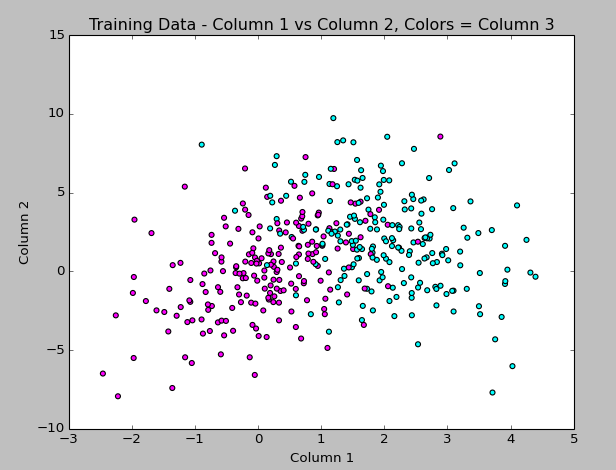
The code to generate this is:
#matplotlib, pyplot, numpy
import matplotlib.pyplot as plt
import numpy as np

#get data from training file
data = np.genfromtxt('train.txt', delimiter = ' ',
          dtype="float, float, int", names = "col1, col2, col3")

#set up color map
import matplotlib.colors as col
import matplotlib.cm as cm
my_colors = ["magenta","cyan"]
my_cmap = col.ListedColormap(my_colors[0:len(my_colors)], 'indexed')
cm.register_cmap(name="mycmap", cmap=my_cmap)

#plot column 1 vs 2 and use column 3 value to apply color
plt.scatter(data["col1"],data["col2"], c=data["col3"], cmap=cm.get_cmap("mycmap"))
plt.title("Training Data - Column 1 vs Column 2, Colors = Column 3")

#label axes and display
plt.xlabel("Column 1")
plt.ylabel("Column 2")
plt.show()
(Hey look at that… syntax highlighting via the Crayon plugin!)
I continued, and picked SciKit-Learn to do the automated Naive Bayes (I have to rewrite a function to do this myself for the project, but wanted to see how it should look). The classifying seemed to work without too much trouble, but colorizing the scatterplot points using matplotlib did not work the way I expected, so that part took the longest to figure out!
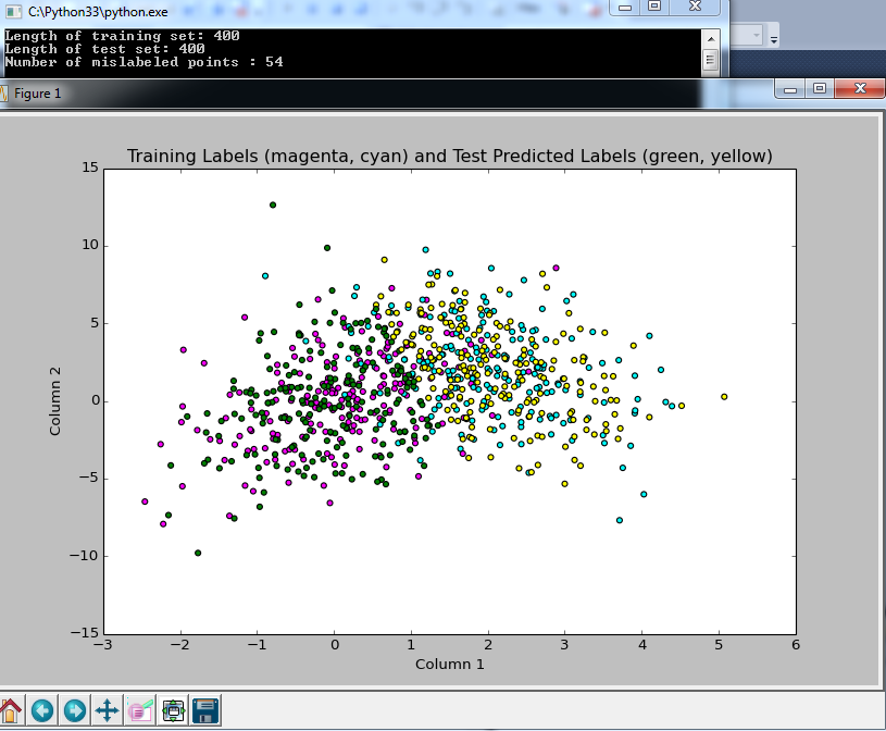
Here I plotted the results of the predicted boolean labels on the test data set based on the Naive Bayes model trained on the Train data set (both data sets provided by my professor). I know it’s not totally clear what I’m doing here, but the image shows the training data in magenta and cyan, with the test data overlayed, colored yellow or green based on the predicted class. I figure it’s a good sign that they overlap like this!
and here is the code:
#example from: http://scikit-learn.org/stable/modules/naive_bayes.html
#from sklearn import datasets
#iris = datasets.load_iris()
#from sklearn.naive_bayes import GaussianNB
#gnb = GaussianNB()
#y_pred = gnb.fit(iris.data, iris.target).predict(iris.data)
#print("Number of mislabeled points : %d" % (iris.target != y_pred).sum())

import numpy as np

#bring in data from files
ftrain = open("train.txt")
ftest = open("test.txt")
data_train = np.loadtxt(ftrain)
data_test = np.loadtxt(ftest)
#can't define 3rd column as integer, or it will collapse to 1D array and next line won't work?
Xtrn = data_train[:, 0:2]  # first 2 columns of training set
Ytrn = data_train[:, 2]  # last column, 1/0 labels
Xtst = data_test[:, 0:2]  # first 2 columns of test set
Ytst = data_test[:, 2]  # last column, 1/0 labels
print("Length of training set: %d " % len(Xtrn))
print("Length of test set: %d " % len(Xtst))

#NAIVE BAYES WITH SCIKIT LEARN
from sklearn.naive_bayes import GaussianNB
gnb = GaussianNB()
#array of predicted labels for test set based on training set?
y_prediction = gnb.fit(Xtrn, Ytrn).predict(Xtst)
#print(y_prediction)
GaussianNB()
print("Number of mislabeled points : %d" % (Ytst != y_prediction).sum())

import matplotlib.pyplot as plt

#set up colors
import matplotlib.colors as col
import matplotlib.cm as cm
my_colors = ["magenta","cyan","green","yellow"]
my_cmap = col.ListedColormap(my_colors[0:len(my_colors)], 'indexed')
#had to add these bounds and mynorm in order to use color indexes below the way I expected it to work
bounds=[0,1,2,3,4]
my_norm = col.BoundaryNorm(bounds, my_cmap.N)
#register the color map with name mycmap
cm.register_cmap(name="mycmap", cmap=my_cmap)

#converting 3rd column to int to use as color index in scatterplot
import array
data_color = array.array('i')
for yitem in data_train[:, 2]:
    data_color.append(int(yitem))
#bring in test data in to view it, adding 2 to the labels get the 3rd and 4th colors from the map
data2_color = array.array('i')
for yitem in y_prediction:
    data2_color.append(int(yitem + 2))

#plot column 1 vs 2 and use 3 to apply color
plt.scatter(data_train[:, 0],data_train[:, 1], c=data_color, cmap=cm.get_cmap("mycmap"), norm=my_norm)
plt.title("Training Labels (magenta, cyan) and Test Predicted Labels (green, yellow)")
#plot column 1 and 2 in test data with different colors based on prediction
plt.scatter(data_test[:, 0],data_test[:, 1], c=data2_color, cmap=cm.get_cmap("mycmap"), norm=my_norm)
#plt.colorbar()
plt.xlabel("Column 1")
plt.ylabel("Column 2")
plt.show()
The output from the classifier says that only 54 data points (out of 400) were not classified properly, based on comparing the predicted label to the true label provided in the test file. Sounds good to me!
So at this point, I’ve only just started the project, but I’m getting more used to Python, and feel like I’m making some progress. I have homework for another class that I’ll probably spend most of tomorrow doing, but I’ll be back this week updating as I continue this project.
Again, I’m not soliciting any help at the moment since I want to do this project on my own if at all possible, but after I turn it in on Thursday, I’d love any advice you have about improving the approach!
]]>The class to date has been mostly “math review” (which is not a review at all for me) and doing homework problems that take 4 pages of work to solve, such as “Show that the Gamma distribution is appropriately normalized”. Needless to say, I’m terrified of the impending midterm I have to take in about a month.
But in the meantime, we just got assigned our first project, having to do with Bayesian Classification! It’s due in 2 weeks and I barely know Python (we can choose any language for this project, and Python is one I’ve been wanting to learn and eventually master since it seems to be used frequently for Data Science work), and barely understand the Bayes classifier, but I’m still excited since learning how to do tasks like this are why I signed up for the class.
Here’s the full description of the project:
Given a training data set and a testing data set (text files), design different classifiers based on the training data set and test the designed classifiers on the test data set.
1. Bayes Classifier: Assume a Gaussian distribution for each class using maximum likelihood to estimate the conditional distribution P(x|ci) and p(ci). Then use Bayes Theory to compute the posterior probability.
2. Naive Bayes Classifier: Assume Gaussian Distribution for each class and assume conditional independence for each variable. Use maximum likelihood to estimate parameters and design a classifier.
3. Use nonparametric method, kernel method, to estimate p(x|ci), use maximum likelihood to estimate p(ci), and design a Bayes Classifier. Determine a suitable value for “h”.
4. Use K-Nearest-Neighbor method to classify the testing data using different k values.
5. Compare your results.
I think this is a lot to do in 2 weeks, especially since we have another difficult homework due in 1 week in this class, and I have homework for another class as well, but I’m going for it!
I had already installed Python into Visual Studio (which I already use for .NET development), and last night I installed scipy, mathplotlib, and numpy along with all of their dependencies. We’re not allowed to use pre-built functions and have to write our own classifiers, but I figure it can’t hurt to have a plan to check all of my work with something established!
My first triumph was importing the data from a text file, discovering it contained 3 columns of data, and creating this 3D plot last night:
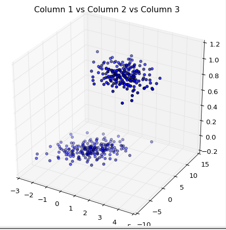
Here’s the code for my first-ever scatterplot in three dimensions:
import matplotlib.pyplot as plt
import numpy as np#get data from training file
data = np.genfromtxt(‘train.txt’, delimiter = ‘ ‘,
dtype=”float, float, float”, names = “col1, col2, col3”)#plot columns 1,2,3 as 3d scatterplot
from mpl_toolkits.mplot3d import Axes3D
import pylab
fig = pylab.figure()
ax = Axes3D(fig)
ax.scatter(data[“col1”],data[“col2”],data[“col3”],zdir=’z’)
plt.title(“Column 1 vs Column 2 vs Column 3”)
plt.show()
(note to self, get a syntax-highlighting wordpress plugin!)
Don’t tell me how to do any of this, since I don’t want to cheat! I’ll post my progress as I go along (though I won’t be back to working on this for about a week since the other homework is due first). Once I’m done with it, I’ll ask for feedback from those of you that know how I could have done it better, so I can keep learning.
I’m excited, and feeling time-crunched!
]]>Short Term (2014-2015):
Get an A in the graduate-level Machine Learning class I’m taking– Done. Got an A!- Finish the activities from the O’Reilly short-course, Udacity course, and Doing Data Science book (more about these later)
Complete the Codecademy Python courseDone! [review]- Learn how to use IPython and Pandas [know basics of both, more to learn!]
- Publish/share a project on GitHub
Complete a machine learning project that helps the University I work for better understand a subset of its data– Partially complete with Machine Learning class Final Project.
Update 1/7/2015: My recently-approved “capstone” project for my masters degree will fulfill this goal!
Longer Term (2014-2017):
Complete my Master’s degree in Systems Engineering (planned for Spring 2015)Done!!- Conduct a thorough study of the data at the University I work for using skills gained in my Data Science coursework to complete an analysis that can help the University raise more money during a fundraising campaign
Update 10/15/15: I have received some funding to help my department learn more about how we can apply predictive analytics and data mining as part of what we do for the university! - Become known for a University Advancement (Development/Fundraising) data science-related achievement (present my work at a CASE conference, for instance)
- Compete in a Kaggle competition or other challenge where my work is compared to others
- NEW GOAL Oct 2015: Build an awesome data science learning directory that uses data science techniques to recommend content to users to help others learn data science! Working on this at DataSciGuide.com
Long Term:
- Get to the point where I have enough skills and projects under my belt to call myself a Data Scientist (I’m aware this is quite subjective), probably with a specialty in University Advancement data
- If it seems necessary/valuable, get a Data Science certification such as the one at Cloudera
- Win a Kaggle competition
- Lead a team of Data Scientists in some way
When I was searching for a graduate degree to pursue, I knew I wanted something technical that could be applied broadly, and which tied in with my love of data, analysis, and studying how things work, without being either an IT/Database Management type program or a pure Computer Science program. Systems Engineering seemed to fit the bill because of its crossover with many fields I wanted to learn more about: computer science, artificial intelligence, cognitive science, human factors, decision theory, modeling & simulation, etc., and because I had enjoyed the introductory engineering courses I took in undergrad. The focus of the Master’s degree seemed to be “how to understand a system and make decisions about it”, which I liked, and thought would be especially applicable to a career incorporating databases in whatever industry I decided to settle into.
What I found out when I got further into the program was that this university’s version of Systems Engineering is VERY math-heavy. I had taken Linear Algebra from a community college as a prerequisite, and took graduate-level Statistics for Scientists and Engineers as part of the program, and had gotten As in both, but soon found myself in courses such as Convex Optimization which were using matrix calculus and other math I never imagined I’d be doing. (An actual Systems Engineer I talked to said that their company would never expect a Systems Engineer to perform these calculations.)
Learning this content was especially challenging because I’m in the program as a “synchronous online” student, meaning that I sit in on the classroom via the web after (or often during) work, and it is difficult to collaborate with other students or get additional help from the professors. (Luckily, my husband is a physicist, so I have an at-home tutor for those times when I get really stuck on my homework!) I started having second thoughts about whether the program was really what I wanted to do, and how it would help my career, I realized that if I wanted this degree to be useful for my life (and maintain the motivation to complete it), I’d need to focus this effort to learn advanced mathematics into something in which I was truly interested.
Around this time, I started hearing more about something called “Data Science”. I read about how Data Science was used in the Obama presidential campaign. I learned about the Netflix Prize, a contest where people built algorithms which could improve the accuracy of movie recommendations. I followed data scientists on twitter to see what it was they did and talked about. I absorbed all of the information I could about this field, and came to realize that 1) I really loved the idea of becoming a Data Scientist, and 2) it wasn’t a big stretch to mold my Systems Engineering degree to have a Data Science focus. (Also around this time, my university announced that they would be starting an MS in Data Science, but it would start as a full-time 11-month program, and not available to students in my distance-learning program, so it wasn’t an option for me.)
The more I read about the field of Data Science, the more it felt like my whole education and career path up to this point had been leading me toward it. I have some formal education in programming and statistics, along with a career in data analytics. I pride myself on having a good grasp of both the business side of data and the technical side of working with it. I was already fascinated with the possibilities surrounding the fast-growing field, and it also didn’t hurt that articles were being published showing how much money a good data scientist could make ($100K+), though that wasn’t my primary motivation. It seemed wise to steer my Systems Engineering Masters Degree to include as many Data-Science-related courses as possible, as “Data Scientist” came into focus as my dream career.
So, I signed up to take a Machine Learning course the next semester which would count as an elective toward my degree, bought some Data Science books, signed up for some online self-paced classes, and got started! I’m about a month into the Machine Learning course now, and we’re about to start our first project, so I decided to start this blog to track my activities and document the hurdles and achievements along the way. I’ll use it as a reference for myself to keep track of resources I find useful, and have a record of the projects I’ve completed. I hope it is interesting enough for others to enjoy reading, and I also hope it provides a sort of “path forward” for those interested in Becoming a Data Scientist, too!
To learn more about my “starting point” on this journey, see the “About Me” page.
I’d appreciate if you fill out a comment below telling me what brought you here, and what you look forward to reading about on this blog!
]]>