Here’s a video of me explaining the analysis:
A few notes as I skim through:
- That part that was broken is where I hadn’t changed from the real IP to the random IP (sorry search bot), so I fixed that in the file below
- I pointed to the wrong thing when I was talking about how long I’d been around…Becoming a Data Scientist Podcast started in December 2015! So 1 year later there was a day larger than the 1st day for the 1st 3 episodes.
- The top IP that got 36 views – I’ll have to look into it, but I think it could be multiple IPs getting assigned the same random number. I’ll take a look and come back when I have a chance.
Here are all of the episodes, so you can go back and listen to any you missed!
You can download the HTML versions of my Jupyter notebooks, and also play with the Tableau dashboards at these links:
“Clean” version of the Jupyter notebook
Full messy analysis Jupyter notebook
Listen monitoring Tableau dashboard
Interactive episodes by week Tableau dashboard
If you have suggestions for how to do the code in a more sensible way than how I rushed and did it, or if you have any questions, feel free to add suggestions in the comments below!
]]>I outlined my whole plan here on my Patreon Campaign. You’ll see a new page on this site soon acknowledging supporters, and I’ll update you on the progress.
Whether you can give financially, or even if you just share the campaign with your data science friends, you are helping Becoming a Data Scientist podcast, the learning club, Data Sci Guide, Jobs for New Data Scientists, and all of my websites get off the ground! Thank you!!
95% of the 158 respondents who gave answers about their jobs follow at least one of my twitter accounts, so you can think of these results as representing my twitter followers.
I’m mostly going to let the tables and graphs speak for themselves. There’s a lot to unpack in the survey (over 50 questions), and a ton of ways to slice and dice it. Because I wanted to show various breakdowns, I did this in simple Excel pivot tables and didn’t spend a ton of time formatting (I know they’re kinda ugly – sorry).
If any of the tables or charts below are particularly hard to understand, please let me know and I’ll annotate further or improve! Click to view full-size.
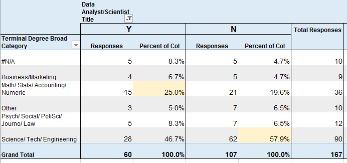
Educational Field
vs Job Title of Data Analyst or Data Scientist (yes/no)
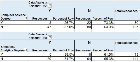
Computer Scientist or Data Sci / Statistics / Analytics Degree
vs Job Title of Data Analyst or Data Scientist (yes/no)
30 (19%) of respondents had CS degrees, which was the most common degree name, and 27% of them had a job title that I categorized under Data Analyst or Data Scientist.
8.3% of respondents had Data Science, Statistics, or Analytics degrees, and 38.5% of them had job titles that I categorized as Data Analyst/Scientist.
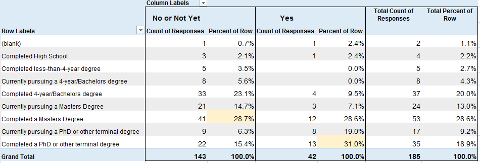
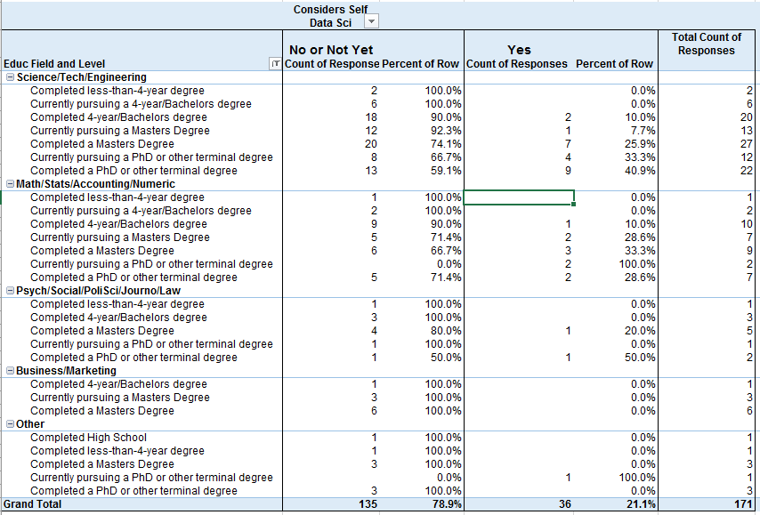
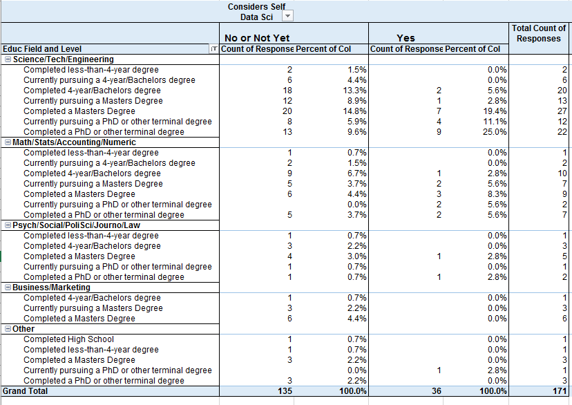
Educational Level
vs Considers Self Data Scientist (No/Not Yet or Yes)
Considers Self Data Scientist by Educational Level and Field
Educational Field by Considers Self Data Scientist
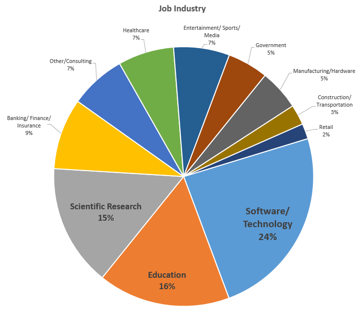
Respondent Breakdown by Job Industry
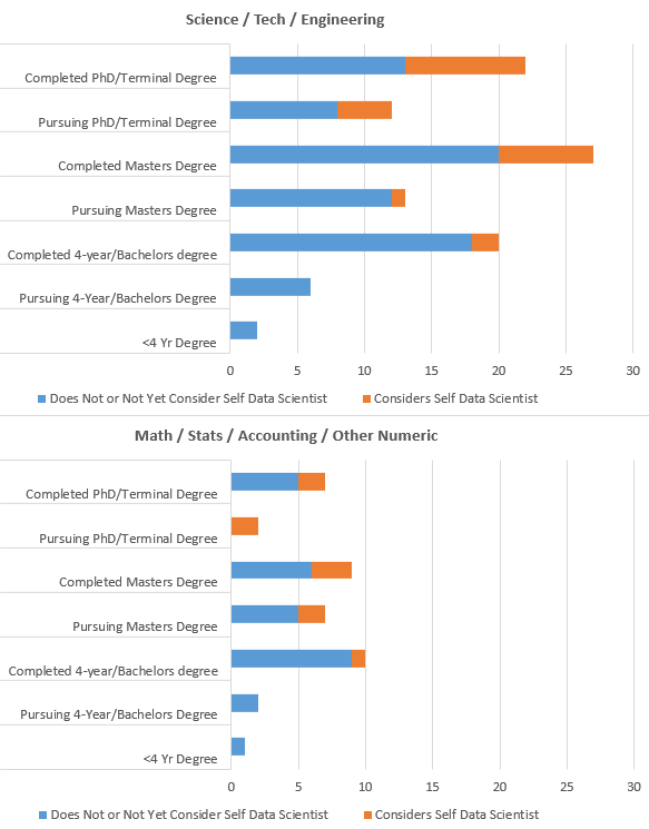
Visual of those with Science/Tech/Eng Degrees and Math/Stats/Acctg Degrees
Percentage of Respondents by “Considers Self Data Scientist” with each Salary Range
About 20% (28) of those that do not consider themselves to be Data Scientists make $50-75K. About 17% (7) of those that do consider themselves to be Data Scientists make under $25K.
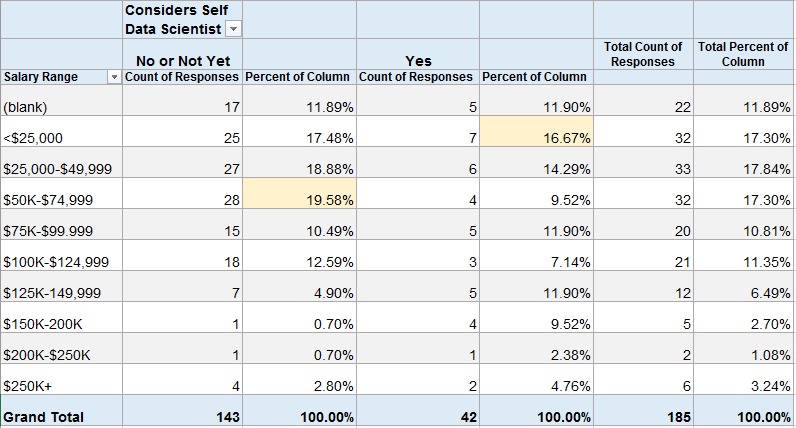
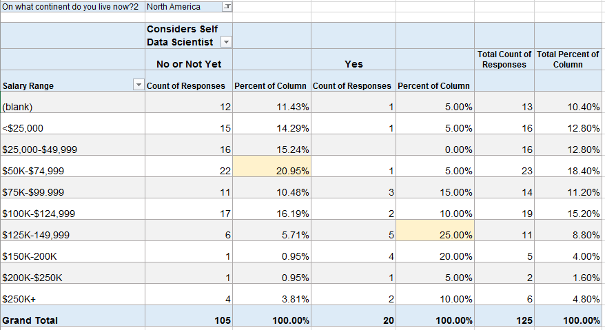
Because the numbers above looked surprising to me, I filtered the same table to those in North America (assuming that many of the low-salary data scientists might be outside of the U.S.).
In North America, about 21% (22) of those that do not consider themselves to be Data Scientists make $50-75K. But now 25% (5) of those that do consider themselves to be Data Scientists make $125-150K. This also shows that 22 of the 42 people above (52%) that considered themselves Data Scientists live outside of North America.
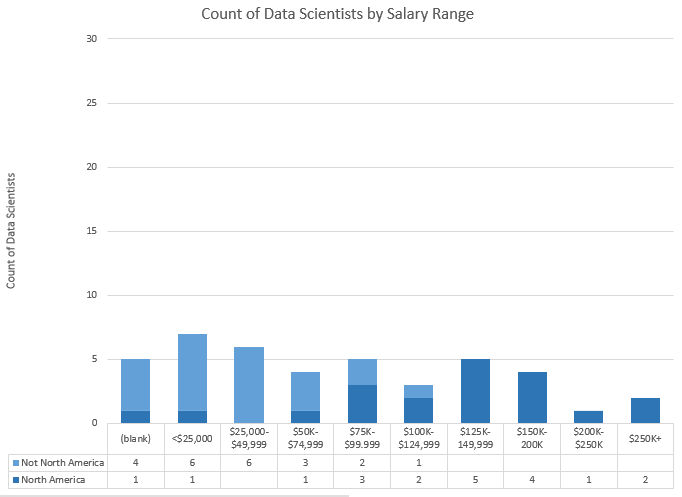
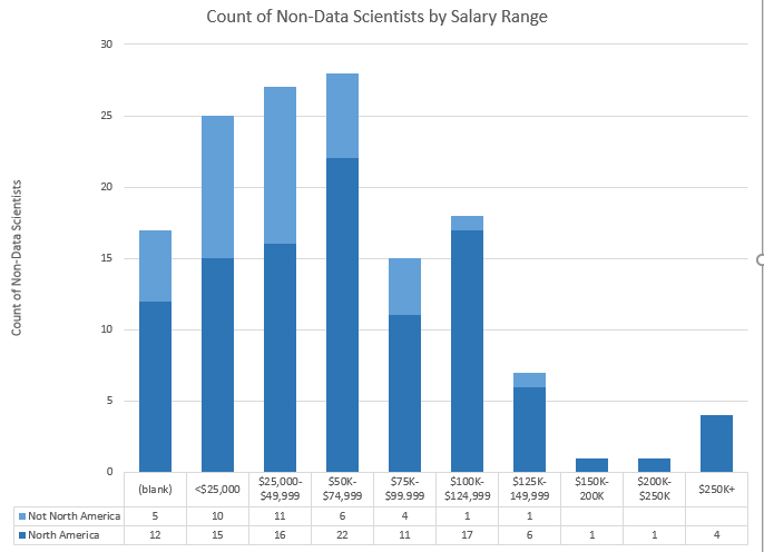
Bar Charts of Above Data. Top = Data Scientists, Bottom = Not Data Scientists.
I may release some of this data at the end of my analysis. If you’re interested in diving in yourself, let me know in the comments and I’ll work on it for a future post.
More results on the way in the near future! Next up, how many respondents follow each twitter account and whether more people watch or listen to the podcast!
]]>
Please fill out the survey and share it with your friends and followers on social media! The survey is a little long/detailed, but most of it is optional. I value your opinions! Thank you so much for participating!!
]]>The first activity involved setting up a development environment. Some people are using R, some using python, and there are several different development tools represented. In this thread, several people posted what setup they were using. I posted a “hello world” program and the code to output the package versions.
Activities 1-3 built upon one another to explore a dataset and generate descriptive statistics and visuals, culminating with a business Q&A:
- Activity 1 – Find & Explore a Dataset
- Activity 2 – Visuals for Exploratory Data Analysis
- Activity 3 – Business Questions & Data Answers
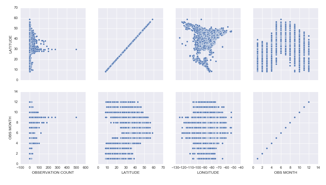
I analyzed a subset of data from the eBird bird observation dataset from Cornell Ornithology for these activities. Some highlights included:
– Learning how to use the pandas python package to explore a dataset (code)
– Learning how to create cool exploratory visuals in Seaborn and Tableau. Here is an example scatterplot matrix made in Seaborn:
– I was most excited to learn how to build interactive Jupyter Notebook inputs, which I used to control Bokeh data visualizations to display Ruby-Throated Hummingbird migration into North America (notebook). Unfortunately, until I host them on a server where you can run the “live” version, you won’t be able to see the interactive widgets (a slider and dynamic dropdowns), but you can see a video of the slider working here:
Here’s my final output for Activity 3, a Jupyter Notebook (with code hidden, and unfortunately interactive widgets disabled) with the Q&A about the hummingbird migration:
Ruby-Throated Hummingbird Migration into North America

Activity 4 was built as a catch-up week for those of us who were behind, but had some ideas of math concepts to learn for those who had time.
We’re currently working on Activity 5, our first machine learning activity where we’re implementing Naive Bayes Classification.
All of my work is available in this github repository: https://github.com/paix120/DataScienceLearningClubActivities
I strongly encourage you to click through the forums and look at some of the other data explorations the members have been doing, including analysis of NFL data, personal music listening habits, transportation in London, German Soccer League data, top-grossing movies, and more!
It’s never too late to join the Data Science Learning Club! If you aren’t sure where to start, check out the welcome message for some clarification.
I’ll post again when I complete some of the machine learning activities!
]]>I had an idea today that would take it a step further. Imagine how book clubs work where you pick a book, go off and read it, then gather occasionally to discuss and record your thoughts. Except instead of a book club, it’s a data science learning club!
I’m imagining picking a topic/project, finding resources showing how to do it, and introducing it to the club at the end of a podcast episode. Then, everyone that wants to participate in learning how to do that particular thing will go off for maybe 2 weeks, work on it and learn what they can, ask questions to each other in a common area like a blog post comment thread, create things and post them to a shared space, then at the end of the period post comments about what they learned and how it went. People could write blog posts about their projects and I would collect those and link to all of them from the original post. Anyone that already knows how to do it could help answer questions if they wanted to participate, too. I might invite some of the participants to talk about their learning experience on a follow-up episode, then the notes and results would be posted for future learners to find.
I think learning together would be fun and valuable, and this type of experience would fall somewhere between learning on your own and taking a class. It would include the pros of learning on your own and exploring, while offsetting some of the cons of going at it alone. It would be a significant time commitment on my part, so I want to make sure other people would join in before I commit. What do you think? Would you join a “data science learning club” and participate in something like this and find it valuable? It’s kind of like the Summer of Data Science, but we’d be learning the same things simultaneously and sharing our results. No one would be “teaching” the group necessarily, but we’d share resources and answer each other’s questions based on what we did individually.
Let me know in the comments or on twitter if you would find this valuable and if you want me to lead it!
]]>Thanks to Orlando and Herbierto for having me on!
(P.S. I did put up the post about Data Sources on DataSciGuide)
]]>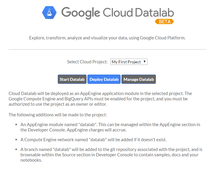
I had a few frustrations with it because the documentation isn’t great, and also sometimes it would silently timeout and it wasn’t clear why nothing was running, but if I stopped all of the services, closed, restarted DataLab, and reopened, everything would work fine again. It’s clearly in Beta, but I had fun learning how to get it up and running, and it was cool to be able to write SQL in a Jupyter notebook.
I tried to connect to my Google Analytics account, but apparently you need a paid Pro account to do that, so I just connected to one of the built-in public datasets. If you view the notebooks, you will see I clearly wasn’t trying to do any in-depth analysis. I was just playing around and getting the queries, dataframes, and charts to work.
I hadn’t planned to get into too many details here, but wanted to share the results. I did jot down notes for myself as I set it up, which I’ll link to below, and you can see the two notebooks I made as I explored DataLab.
Exploring BigQuery and Google Charts
Version Using Pandas and Matplotlib
(These aren’t tidied up to look professional – please forgive any typos or messy approaches!)
Google Cloud Datalab Setup Notes (These are notes I jotted down for myself as I went through the setup steps. Sorry if they’re not intelligible!)
]]>Here’s more info: http://www.datasciguide.com/review-stuff-and-win-a-40-amazon-gift-card/
]]>That site isn’t open for comments yet, so I’m directing people to leave feedback here.
If you haven’t kept up with the development of DataSciGuide, here are a few things to read:
Let me know if you want an account to post some reviews while I test things out! (I’ll even post content that you want to review, just for you.)
Also, tell me any thoughts you have about the site in the comment form below! (or tweet me!)
]]>My main motivation is that I keep hearing people say (and sometimes feel myself) that learning to becoming a data scientist on your own using online resources is totally overwhelming: there are so many different possible topics to dive into, few really good guides, lots of impostor-syndrome-inducing posts by people you follow that make you feel like they’re so far ahead of where you are and you’ll *never* get there…. but there’s so much great data science learning content online for everyone from beginners to experienced data scientists!
We need a better way to navigate it.
Hence my new website: “Data Sci Guide”. It will eventually have a personalized recommender system and structured learning guides and all kinds of other features to help you find the resources to go from where you are to where you want to be, but for now it’s “just” a directory / content rating site. And it’s not ready for you to interact with yet, but it’s getting there, and I’ll need your help fleshing it all out soon.
So go take a look! Then come back here to give me feedback and suggestions, because you have to be registered to comment there and I didn’t turn on new user registration yet.
OK go now. Don’t forget to come back!

>>>> DATA SCI GUIDE.COM <<<
So…. what did you think? What do you think of the overall idea and plans? What should I be sure to remember to include? Tell me below!
]]>
I posted earlier about using the UsesThis API to retrieve data about what other software people that use X software also use. I thought I was going to have to code a workaround for people that didn’t have any software listed in their interviews, but when I tweeted about it, Daniel from @usesthis replied that it was actually a bug and fixed it immediately! It makes it even more fun to develop since he is excited about me using his API!
@BecomingDataSci: YES! It’s *awesome*.
— The Setup (@usesthis) June 19, 2015
After seeing those results, I thought it would be interesting (and educational) to learn how to do a Market Basket Analysis on the software data. Market Basket Analysis is a data mining technique where you can find out what items are usually found in combination, such as groceries people typically buy together. For instance, do people often buy cereal and milk together? If you buy taco shells and ground beef, are you likely to also buy shredded cheese? This type of analysis allows brick and mortar retailers to decide how to position items in a store. Maybe they will put items regularly purchased together closer together to make the trip more convenient. Maybe they will place coupons or advertisements for shredded cheese next to the taco shells. Or maybe they will place the items further apart so you have to pass more goods on the way from one item to the other and are more likely to pick up something you otherwise wouldn’t have. Online retailers can use this type of analysis to recommend products to increase the size of your purchase. “Other customers that added item X to their shopping cart also purchased items Y and Z.”
Because I had this interesting set of software usage from The Setup’s interviews, I wanted to analyze what products frequently go together. I searched Google for ‘Market Basket Analysis python,’ and it led me to this tweet by @clayheaton:
I just wrote a simple Market Basket analysis module for Python. #analytics https://t.co/aVf58zcHJa
— Clay Heaton (@clayheaton) April 4, 2014
I followed that link and checked out the code on github and it seemed to make sense, so I put the results of my usesthis API request into a format it could use. I did a test with the data from 5 interviews, and it ran. Then I tried 50 interviews, and the results showed that people that use Photoshop were likely to also use Illustrator, and vice-versa. It appeared to be working!
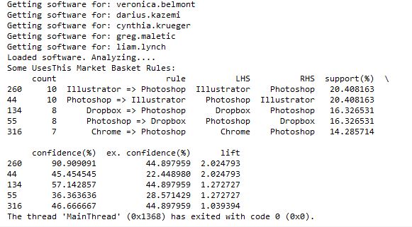
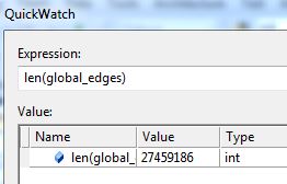
However, I then hit a snag. I tried to run it with all of the software data, and it ran for a long time then crashed when my computer ran out of memory. Since it’s building an association graph with an edge for every rule (combination of software used), with up to two pieces of software per “side” of the rule (such as “people that have Photoshop and Illustrator also have a Mac”), you can imagine the graph gets pretty big when you have over 10,000 user-software combinations.
I tweeted about this and Clay suggested modifying his code to store the items in a sparse matrix instead of a graph, and I agree that that sounds like a good approach, so that’s my next step on this project. I’ll post again when I’m done!
]]>Then, I tweeted about my experience, and got 2 responses encouraging me to use the requests library instead of urllib that codecademy used.
@BecomingDataSci the urllib api is terrible. You should take a look at http://t.co/CzIPob2tBV
— Daniel Moisset (@dmoisset) June 1, 2015
@dmoisset @BecomingDataSci 2nding using of requests over urllib; esp. with HTTPS, requests tends to do saner things (e.g., cert validation)
— Cheng H. Lee (@chenghlee) June 1, 2015
I decided to redo what I had learned from scratch, but using requests. I also wanted to learn how to use IPython, so I used an IPython notebook to play around with the code. Below is the HTML export of my IPython notebook, with comments explaining what I was doing. I’m sure there are better ways to do what I did (feel free to comment with suggestions!), but this was my first time doing any of this without any guidance, so I don’t mind posting it even if it’s a little ugly :) I definitely spent a lot of time understanding the hierarchy of the NPR XML and how to loop through it and display it. If you have done something similar in a more elegant way, please point me to your code!
Here are the main resources I used to learn how to do what is in the code:
- python requests library documentation
- NPR API documentation
- python lxml library documentation
- iPython videos
I also wanted to mention that there are a lot of frustrations you can run up against when you’re a python beginner. I was having a lot of problems with seemingly basic stuff (like installing packages with pip) and it took a couple hours of googling and asking someone for help to figure out there was a problem with my path environment variables in windows. I’ll post about that another time, but I just wanted to 1) encourage people not to give up if you get stuck on something that seems to be so basic that most “intro” articles don’t even cover it, and 2) encourage people writing intro articles to make some suggestions about what could go wrong and how to problem-solve.
Here’s one example: When I tried to export my IPython notebook to HTML, it gave me a 500 server error saying I needed python packages I didn’t already have. After I installed the first, it told me I needed pandoc, so I installed that as well, but it kept giving me the same error. It turns out that you have to run IPython Notebook as an Administrator in Windows in order to get the HTML export to work properly, but the error message didn’t indicate that at all. This is the kind of frustration that may make beginners think they’re not “getting it” and give up, when it fact it’s something outside the scope of what you’re learning. Python seems to require a lot of this sort of problem-solving.
(Note: on my other laptop, I installed python and the scipy stack using Anaconda, and have had a lot fewer issues like this.)
Without further ado, here’s my iPython notebook! (I’m having issues making it look readable while embedded in wordpress, so click the link to view in a new tab for now, and I’ll fix for viewing later!)
Renee’s 1st IPython Notebook (NPR API using requests and lxml)
Here’s the actual ipynb file if you have IPython installed and want to run it yourself: First Python API Usage**
**NOTE: WordPress wouldn’t let me upload it with the IPython notebook extension for security reasons, so after you download it, change the “.txt” extension to “.ipynb”!
select fiscal_year, donorid,
    (case when DonorID IN (select donorid from Donations d1 where d1.fiscal_year = d.FISCAL_YEAR - 1 and HardCredit > 0) then 'Retained'
         when DonorID IN (select donorid from Donations d2 where d2.fiscal_year >= d.FISCAL_YEAR - 5 and d2.FISCAL_YEAR <= d.fiscal_year - 2 and HardCredit > 0) then 'Reactivated 2-5'
         when DonorID IN (select donorid from Donations d3 where HardCredit > 0 and d3.FISCAL_YEAR < d.FISCAL_YEAR - 5 ) then 'Reactivated Lapsed'
         else 'Acquired Donor'
         end)  FY_DonorType
from Donations d
    where Donor_Record_Type = 'A' and HardCredit > 0
    group by fiscal_year, donorid,  (case when DonorID IN (select donorid from Donations d1 where d1.fiscal_year = d.FISCAL_YEAR - 1 and HardCredit > 0) then 'Retained'
         when DonorID IN (select donorid from Donations d2 where d2.fiscal_year >= d.FISCAL_YEAR - 5 and d2.FISCAL_YEAR <= d.fiscal_year - 2 and HardCredit > 0) then 'Reactivated 2-5'
         when DonorID IN (select donorid from Donations d3 where HardCredit > 0 and d3.FISCAL_YEAR < d.FISCAL_YEAR - 5 ) then 'Reactivated Lapsed'
         else 'Acquired Donor'
         end)
         ;
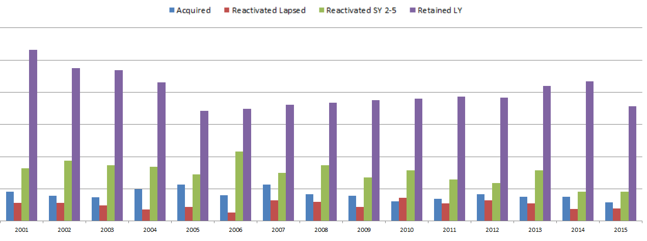
So in the Donations table, there is one row per donor per gift. There can be multiple gifts in a fiscal year, but as soon as the first gift is made, the donor can then be given a FY_DonorType using a CASE statement. If the donor also gave last year, then the donor is “Retained”. If they have given in the past, they’re “Reactivated”. I separated out those reactivated in the last 2-5 years and those that hadn’t given for longer, since once a donor had not given for 5 years, they are considered “Long Lapsed” and much harder to reactivate. If the donor had never appeared in the table before, he or she is a New donor and marked as “Acquired”. We are not looking at how many people gave last year but not this year (“Lost”), but only the breakdown of who this year’s donors are.
Since the code groups by fiscal year and donor ID, and the case statements include selects that look at previous years relative to each gift’s fiscal year, you can look at how the “current year” donors break down every year. Each year is relative to the previous years.
This allows us to make visualizations that give some insight into how the fundraising team performed each year. Some years, the fundraising organization was particularly good at reactivating lost donors. Some years they retained donors from the previous fiscal year at a high rate, but the ones that hadn’t given for more than a year must not have been targeted well and fell off more than usual. This is likely a result of how often they solicited each group, and what type of solicitations were used. (I purposely hid the Y-axis and other info since I’m using this for illustrative purposes and not trying to give away details related to the fundraiser.)
What database tables do you have that could be analyzed in this way?
]]>I had a thought while daydreaming, and tweeted this, thinking a few people might think it was fun and respond:
I'm planning to do a lot of data science learning this summer. Anyone else? Maybe we shld start a hashtag #SoDS "Summer of Data Science" :)
— Data Science Renee (@BecomingDataSci) May 14, 2015
…and as you can see by the RT and Favorite count, it kind of took on a life of its own!
I thought of a variation
…or maybe more fun #SODAS "Summer of Data Science". like a cool, refreshing beverage. & we'll hand off to So Hemisphere ppl in the fall :)
— Data Science Renee (@BecomingDataSci) May 14, 2015
and so did some other people
@BecomingDataSci It could be #SoDaS (just add the little "a" in there for D"a"ta…)
— Nicole Radziwill (@nicoleradziwill) May 14, 2015
@BecomingDataSci #DSS15 Data Science Summer 2015
— BigMikeInAustin (@BigMikeInAustin) May 14, 2015
In the end, it looks like #SoDS won…. and got a whole lot of support because of a RT by @dpatil! Thanks to him, this is what my notifications started to look like:
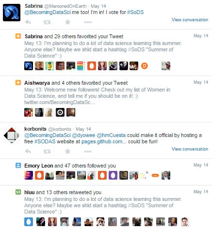
Too bad I was supposed to be working on writing up something for work…. that didn’t get done that night! I came back later and was really surprised by the response!
I was excited by all of the new followers, and especially happy that some people appeared to have been inspired by the hashtag to do some data science learning of their own!
@BecomingDataSci @seinecle and is there something like "data science for über-beginners"? =D
— Lexane Sirac (@lexanesirac) May 14, 2015
2 minutes later…
@BecomingDataSci @seinecle @clarecorthell thank you so much! I'll make sure to take part in #SoDS then!
— Lexane Sirac (@lexanesirac) May 14, 2015
So it seems I started something and now I need to follow up! I’m going to tag my summer learning projects on here with the “#SoDS 2015” post category, and tweet about them (of course!) using the #SoDS hashtag on twitter. Will you join me? :)
Here’s to an awesome Summer of Data Science! Now I’m going to try to go respond to all of your tweets!
(P.S. the hashtag just started being used by some Dutch foodies, but we’ll overwhelm that version with our data science tweets pretty soon!)
P.P.S. we even have a unicorn joining us this summer!
@BecomingDataSci @DataSkeptic count me in! #SoDS #becomingaunicorn
— Data Science Unicorn (@DataScienceUni) May 14, 2015
]]>Principles of Data Visualization for Exploratory Data Analysis [presentation – pdf]
Principles of Data Visualization for Exploratory Data Analysis [paper – [pdf]
Check out the references in both documents for some good resources. I’ll include some links in the post below, too. I had a lot more material from my research that I wanted to include and just didn’t have time to in a 15-minute presentation! The professor was happy about the topic I picked because she’s teaching a class on Data Visualization next semester, so I think that worked out in my favor :)
These two books by Stephen Few covered the very basics of visualization for human perception:
Show Me the Numbers: Designing Tables and Graphs to Enlighten
Now You See It: Simple Visualization Techniques for Quantitative Analysis
Blog posts about related topics:
Six Revisions: Gestalt Laws
eagereyes: Illustration vs Visualization
Detailed visualization of NBA shot selection
Publications and articles:
IEEE Transactions on Visualization and Computer Graphics
Toward a Perceptual Science of Multidimensional Data Visualization: Bertin and Beyond by Marc Green, Ph. D.
Scagnostics by Dang and Wilkinson
Generalized Plot Matrix (GPLOM) by Im, McGuffin, Leung
UpSet: Visualization of Intersecting Sets by Lex, Gehlenborg, Strobelt, et al.
…and there are more resources in the paper and presentation files! (and if you’re REALLY interested in this topic, post a comment and I will add even more links I have bookmarked)
I also did a project using some data from my day job related to university fundraising and major gift prospects, but unfortunately I can’t share that study here because I don’t have permission to do so. It included some cool visuals like bubble charts, and also an interesting analysis of movement through the prospect pipeline using Markov Chains. I learned a lot doing that one!
It was nice to end my final semester of grad school with two data-related projects! (Yes, I’m finally graduating! Masters of Systems Engineering! woo hoo!)
]]>——————————————-
“MANUAL” APPROACH USING EXCEL
So first I started out by seeing if I could create a scoring model in Excel which could be used to classify the patients. I started with the Cleveland data set that was already processed, i.e. narrowed down to the most commonly used fields. I did some simple exploratory data analysis on each field using pivot tables and percentage calulations, and decided on a value (or values) for each column that appeared to correlate with the final finding of heart disease or no heart disease, then used those results to add up points for each patient.
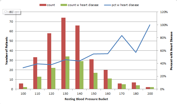
For instance, I found that 73% of patients with Chest Pain Type 4 ended up being diagnosed with heart disease, where no higher than 30% of patients with any other Chest Pain Type ended up with that result. So, the people that had a 4 in the “chest pain type” column got 2 points. For Resting Blood Pressure, I grouped the values into 10-point buckets, and found that patients with a resting blood pressure value of below 150 had a 33-46% chance of being diagnosed with heart disease, where those with 150 and up had a 55-100% chance. So, patients with 150 or above in that column got an additional point.
Points ended up being scored for the following 12 categories:
- Age group >=60
- Sex = male
- Chest Pain Type 4 [2 points]
- Resting Blood Pressure group >= 150
- Cholestoerol >= 275
- Resting ECG > 0
- Max Heart Rate <= 120 [2 points], between 130 and 150 [1 point]
- Exercise-induced Angina = yes [2 points]
- ST depression group >=1 [1 point], >=2 [2 points]
- Slope of ST segment > 1
- Major Vessels colored by Fluoroscopy = 1 [1 point], >1 [2 points]
- thal = 6 [1 point], thal = 7 [2 points]
This was a very “casual” approach which I would refine dramatically for actual medial diagnosis, but this was just an exercise to see if I could create my own “hand-made” classifier that could actually predict anything. So at this point I had to decide how many points merited a “positive” (though not positive in the patients’ eyes) diagnosis of heart disease. I tried score thresholds of between 6 and 9 points, and also tried a percentage-based scoring system, and the result with the most correct classifications was at 8 points. (8+ points classified the patient as likely having heart disease.) However, the 8-point threshold had a higher false negative rate than the lower thresholds, so if you wanted to make sure you were not telling someone they didn’t have heart disease when they in fact did, you would use a lower threshold.
The final results with the 8-point threshold were:
| true positive | 112 | 37% |
| false positive | 18 | 6% |
| true negative | 146 | 48% |
| false negative | 27 | 9% |
| correct class | 258 | 85% |
I remembered that the symptoms for heart disease in males and females could look very different, so I also looked at the “correct class” percentages for each sex. It turns out that my classifier classified 82% of males correctly, and 93% of females. Because of how long it took to create this classifier “the manual way”, I decided not to redo this step to create a separate classification scheme for each sex, but I decided to test out training separate models for men and women when I try this again using Python.
TESTING THE MODEL
I made the mistake of not checking out the other data sets before dividing the data into training and test sets. Luckily the Cleveland dataset I used for training was fairly complete. However, the VA dataset had a lot of missing data. I used my scoring model on the VA data, but ended up having to change the score threshold for classifying, because the Cleveland (training) dataset had rows with an average of almost 11 data points out of 12, but the VA (test) dataset only averaged about 8. So, I lowered the threshold to 6 points and got these results:
| true positive | 140 | 70% |
| false positive | 38 | 19% |
| true negative | 13 | 7% |
| false negative | 9 | 5% |
| correct class | 153 | 77% |
This time, separating out the sexes, it classified only 67% of the females correctly, but 77% of the males. However, there were only 6 females (out of 200 records) in the dataset, so that result doesn’t mean much.
I think classifying 77% of the records correctly is good for a model created as haphazardly as this one was! I learned good lessons about checking out all of the available data before starting to develop a plan for training and testing, and also again encountered an imbalanced dataset like I did in one of my graduate Machine Learning class projects.
——————————————-
AUTOMATED DATA MINING USING PYTHON
Now that I “played around” with creating my own model in Excel, I wanted to use code to create a classifier in Python. I had already written a classifier in Python for one of my other projects in Machine Learning grad class, but wanted to do it more quickly (and probably more correctly) using commonly-used Python packages designed for this type of work.
I decided to learn how to use the Pandas library since I had heard it makes the import and manipulation of data sets much simpler, and try both the Nearest Neighbors and Decision Trees classifiers from scikit-learn.
I had a little trouble getting everything set up the way it needed to be. I eventually got the right versions of the scipy-stack and scikit-learn in Python 3.3. Because I already had it installed and am familiar with it, I’m using Visual Studio as an IDE, but I’m probably going to drop that soon for something leaner. Commenters on Twitter suggested checking out Anaconda/miniconda for easy installs, so I plan to take a look at that soon.
I read the documentation on pandas and scikit-learn and figured out how to import data, manipulate it (For instance, some of the values were question marks. When I made the classifier in Excel (above), I deleted these. This time, I turned them into numeric values because the classifiers couldn’t handle Null values. I need to learn how to best handle these in a future practice session.)
Here is an example of importing the data from the CSV into a pandas dataframe:
#import the Cleveland heart patient data file using pandas, creating a header row
#since file doesn't have column names
import pandas as pnd
header_row = ['age','sex','pain','BP','chol','fbs','ecg','maxhr','eiang','eist','slope','vessels','thal','diagnosis']
heart = pnd.read_csv('processed.cleveland.data', names=header_row)
Here is where I converted the “diagnosis” values in the file to a 1/0 result (any value above 0 was a heart disease diagnosis):
#import and modify VA dataset for testing
heart_va = pnd.read_csv('processed.va.data', names=header_row)
has_hd_check = heart_va['diagnosis'] > 0
heart_va['diag_int'] = has_hd_check.astype(int)
And here is an example of training the Decision Tree classifier, then outputting the results of various tests:
#classification with scikit-learn decision tree
from sklearn import tree
clf2 = tree.DecisionTreeClassifier()
#train the classifier on partial dataset
heart_train, heart_test, goal_train, goal_test = cross_validation.train_test_split(heart.loc[:,'age':'thal'], heart.loc[:,'diag_int'], test_size=0.33, random_state=0)
clf2.fit(heart_train, goal_train )
heart_test_results = clf2.predict(heart_test)

#put the results into a dataframe and determine how many were classified correctly
heart_test_results = pnd.DataFrame(heart_test_results, columns=['predict'])
goal_test_df = pnd.DataFrame(goal_test, columns=['actual'])
heart_test_results['correct'] = heart_test_results['predict'] == goal_test_df['actual']

#print results of decision tree classification test
print("")
print("Decision Tree Result 1:")
print(heart_test_results['correct'].value_counts())
print(clf2.score(heart_test, goal_test))

#try the scikit-learn cross validation function
print("Decision Tree Cross-Validation:")
scores = cross_validation.cross_val_score(clf2, heart.loc[:,'age':'thal'], heart.loc[:,'diag_int'], cv=5)
print(scores)

#test classifier with other data (note: many values missing in these files)
print("Trained Decision Tree Applied to VA Data:")
heart_va_results = clf2.predict(heart_va.loc[:,'age':'thal'])
print(clf2.score(heart_va.loc[:,'age':'thal'], heart_va.loc[:,'diag_int']))
print("Trained Decision Tree Applied to Hungarian Data:")
heart_hu_results = clf2.predict(heart_hu.loc[:,'age':'thal'])
print(clf2.score(heart_hu.loc[:,'age':'thal'], heart_hu.loc[:,'diag_int']))
Interestingly, the results these classifiers got weren’t much better than my “homemade” classifier above! Here is the output from my code:
Nearest Neighbors (5) Result 1:
True 64
False 36
dtype: int64
0.64
Nearest Neighbors (5) Cross-Validation:
[ 0.62295082 0.67213115 0.63934426 0.65 0.7 ]
Trained Nearest Neighbors (5) Applied to VA Data:
0.615
Trained Nearest Neighbors (5) Applied to Hungarian Data:
0.421768707483
Decision Tree Result 1:
True 75
False 25
dtype: int64
0.75
Decision Tree Cross-Validation:
[ 0.7704918 0.75409836 0.73770492 0.8 0.76666667]
Trained Decision Tree Applied to VA Data:
0.65
Trained Decision Tree Applied to Hungarian Data:
0.683673469388
The Nearest Neighbors classifier was able to classify 62-70% of the training data correctly, and only 61% of the VA data.
The Decision Tree classifier was able to classify 73-80% of the training data correctly, and only 65% of the VA data.
My model in Excel classified 85% of the training data correctly and 77% of the VA data (with a change in the “points” system knowing that the VA file had fewer available columns). In this case, a “human touch” appeared to make a difference!
——————————————-
Overall, I learned a lot from this exercise and will definitely revisit it to improve the results and add more analysis (such as true/false positive and negative counts on the scikit-learn results, filling in the null values or removing those rows, and comparing results if the male and female patients are split into separate datasets to train separate models). I enjoyed learning Pandas and look forward to exploring more of what it can do! If you have suggestions for future analysis of this dataset, please put them in the comments. (Also please let me know if I made any glaring mistakes!) I’ll upload my files (linked below) so you can see all of my “playing around” with the data!
(messy) Excel file with my data exploration and point system for classifying
Heart Disease Classification python code(change file extension to .py after downloading — wordpress won’t let me upload as .py for security reasons)
]]>Very good analysis and you showed great potential to become a good researcher!
Comments:
1. when you code your categories features, 1 of k coding is a good choice. Did you apply this method to all categories features?2. Some time, normorlize features will make a huge difference. One way to do this is to comput the z-score for features before you train a model on the data.
3. In terms of machine learning application, your analysis is good. If you try to find a social study expert to collobrate with you, I believe your findings can be published on high impacting journals.
4. In order to publish your work, you will need to do some research to found what have been done in this field.
This is especially encouraging since I want to become a data scientist, so hearing positive feedback like this, even encouraging me to publish after having only taken one semester of Machine Learning, feels great!
So, I will take time this summer to do more research and learning and expand on this project (since it was a rush to complete enough to turn in on time in this class but there’s a lot more I want to do with it), and I will collaborate with some people at the university where I work to further distill the results and see if we can apply them to segment out some potential first-time donors for next fiscal year.
This is fun!
]]>I settled on using SciKit-Learn (skLearn) Random Forest since I have been teaching myself Python throughout this class and kept seeing references to the skLearn package for machine learning. I like their site, and the documentation was good enough to get me started. skLearn also has tools for preprocessing data, which is something I knew I’d need since I was working with a “real world” data set, so I got started.
First, I decided on what problem to tackle. Since this was a classification project, I decided to see if I could identify people that gave to the university for the first time in a fiscal year, and compared “never givers” (non donors) to “first time donors”. I pulled data such as class year, record type (alumni, parent, etc.), college, zip code, distance from the school, whether we had an address/email/phone number for them, whether they were assigned to a development officer, how long their record had been in the database, how many solicitation and non-solicitation contacts they had with the university, whether they were a parent of a current student, had ever been an employee of the university, etc.
Many of these columns were yes/no (like Has Email) or continous (like distance), so didn’t need any modification except figuring out what to do when the field was null. I wrote functions to return values that I thought made sense for when the field was empty, and figured I’d play around with those a bit when I saw the results. I also tried excluding the rows with empty values in certain columns, but that made the result worse.
So, when I first ran the Random Forest (the code for this part was the easiest part of the project thanks to skLearn!), the scores looked like this:
Overall score: 98%
Class 0: 99%, 141,500 records
Class 1: 16%, 2,300 records
Class 0 had all of the records of everyone that had ever been added to our database for any reason but had not made a gift to the university, while class 1 consisted only of people who had made their first gift in Fiscal Year 2013. As you can see, I learned a lesson about working with an imbalanced dataset.
I learned how to output the “importances” of each column that the Random Forest used to classify the data and started manipulating my dataset. First, I tried “downsampling”, which means that you remove some records from the larger class so it doesn’t contribute so heavily to the results. I also brought in more fields that were categorical, such as the Record Type Codes, and used the skLearn Preprocessing functions “LabelEncoder”, which turned the string categories into numerical values, and “OneHotEncoder”, which then turned those numerical values into 1-of-k sparse arrays with the column value a 1 and every other value a 0. For instance, “AL” for Alumni would be category “1”, and encoded as [1 0 0 0 0 0 0 0 0] if there were 9 possible categories.
Eventually, I got the results to look like this:
Overall score: 99%
Class 0: 99%, 101,750 records
Class 1: 97%, 2,032 records
Now, there are some “wrong” reasons that I could have come out with such good results, so to better understand this (and to be able to use these results to provide any insight to the Office of Annual Giving), I need to figure out how to output the values that the Random Forest is using to classify each point (not just the weights of the columns). I am pretty sure there is a way to do this, but I just didn’t have time during this 2-week project which I mostly worked on late-night while working full time (luckily my manager gave me 2 days off during the final 2 weeks to work on this final project and another for my Risk Analysis class since they were each 30% of my grade). So, that will be my next step in learning how to better work with this type of data.
Additionally, I want to learn how to output some visualizations, such as a “scatter matrix” which plots each column in a dataset against every other column so you can visually spot which have strong correlations. (I plan to learn how to do that using this: Pandas Scatter Plot Matrix)
I also tried to see if my FY13 data could be used to predict FY14 first-time donors. There are some good reasons it wasn’t perfect, but it appears I was able to correctly classify 67% of the data points for first time donors, which I don’t think is too bad.
I have attached my project write-up and some python code if anyone wants to take a look. I can’t attach the dataset because of privacy and permission issues, but a sample row looks like this:
DATA_CATEGORY: FIRST TIME DONOR FY13
CLASSIFICATION: 1
FY14 RECORD TYPE: AL
YEARS_SINCE_GRADUATED: 2
PREF_SCHOOL_CODE: COB
OKTOMAIL: 1
OKTOEMAIL: 1
OKTOCALL: 1
EST_AGE: 24
ASSIGNED: 0
ZIP5: 23219
ZIP1: 2
MI_FROM_HBURG: 98.65
HAS_PREF_ADDRESS: 1
HAS_BUSINESS_ADDRESS: 0
HAS_PHONE: 0
HAS_EMAIL: 1
FY1213_SOLICIT_B4: 2
FY1213_NONSOLICIT_B4: 5
FY1213_SOL_NONOAG_B4: null
FY1213NONSOLNONOAGB4: 4
SOLICITATIONS: 2
NONSOLICITAPPEALS: 5
CURRENT_RECENT_PARENT: 0
EVER_EMPLOYEE: 0
YEARS_SINCE_ADDED: 1.00
YEARS_SINCE_MODIFIED: null
EVENT_PARTICIPATIONS: 0
Any feedback is welcome! I am very relieved that this semster is done, and I plan to spend the summer learning as much as possible about Data Science topics, so throw it all at me! :)
(Again, I have to change the .py file extensions to .txt for wordpress to allow me to upload)
607 ML Final Project Write-Up
So, to wrap up Project 3. I ended up getting the Neural Networks working in PyBrain, but when it came to Support Vector Machines (SVM), I just could not get it to run without errors. I had already downgraded to Python 2.7 to get PyBrain working at all, but there were further dependencies for the SVM functionality, and at midnight the night before it was due, I still hadn’t gotten it to run, so I figured it was time to try another approach. This is when I started looking at SciKit-Learn SVM.
I had wanted to do the whole project in PyBrain if possible, but it turned out that switching to SciKit-Learn (also called sklearn) was a good idea, because the documentation was helpful and the implementation painless. I had to tweak how I was importing the data from the training and test files since I was no longer using PyBrain’s ClassificationDataSet, but that wasn’t a complicated edit.
I was able to implement both the RBF and Linear kernel versions of the SVM Classifier (called SVC in sklearn). The Linear one actually worked better on the test data provided by the professor, and it correctly classified 96% of the data points (which were evenly split into 2 classes). In addition, I was able to make these cool plots by following the instructions here.
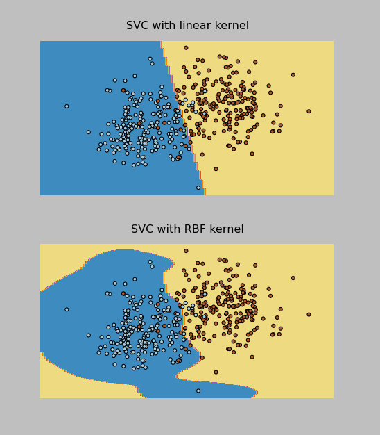
I have pasted the SVM code below and attached all of my project files to this post. Now on to the Final Project, due May 9.
Thanks to everyone that gave me tips on Twitter while I was working through the installations on this one!
import pylab as pl
import numpy as np
from sklearn import svm, datasets

print("\nImporting training data...")
#bring in data from training file
f = open("classification.tra")
inp = []
tar = []
for line in f.readlines():
    inp.append(list(map(float, line.split()))[0:2])
    tar.append(int(list(map(float, line.split()))[2])-1)


print("Training rows: %d " %  len(inp) )
print("Input dimensions: %d, output dimensions: %d" % ( len(inp), len(tar)))
#raw_input("Press Enter to view training data...")
#print(traindata)
print("\nFirst sample: ", inp[0], tar[0])

#sk-learn SVM
svm_model = svm.SVC(kernel='linear')
svm_model.fit(inp,tar)

#show predictions
out = svm_model.predict(inp)
#print(test)
class_predict = [0.0 for i in range(len(out))]
predict_correct = []
pred_corr_class1 = []
pred_corr_class2 = []
for index, row in enumerate(out):
    if row == 0:
        class_predict[index] = 0
    else:
        class_predict[index] = 1
for N in range(len(class_predict)):
    if class_predict[N] == tar[N]:
        if tar[N] == 0:
            pred_corr_class2.append(1)
        if tar[N] == 1:
            pred_corr_class1.append(1)
        predict_correct.append(1)
    else:
        if tar[N] == 0:
            pred_corr_class2.append(0)
        if tar[N] == 1:
            pred_corr_class1.append(0)
        predict_correct.append(0)

print ("SVM Kernel: ", svm_model.kernel)
print ("\nCorrectly classified: %d, Percent: %f, Error: %f" % (sum(predict_correct),sum(predict_correct)/float(len(predict_correct)),1-sum(predict_correct)/float(len(predict_correct))))
print ("Class 1 correct: %d, Percent: %f, Error: %f" % (sum(pred_corr_class1),sum(pred_corr_class1)/float(len(pred_corr_class1)),1-sum(pred_corr_class1)/float(len(pred_corr_class1))))
print ("Class 2 correct: %d, Percent: %f, Error: %f" % (sum(pred_corr_class2),sum(pred_corr_class2)/float(len(pred_corr_class2)),1-sum(pred_corr_class2)/float(len(pred_corr_class2))))


raw_input("\nPress Enter to start testing...")

print("\nImporting testing data...")
#bring in data from testing file
f = open("classification.tst")
inp_tst = []
tar_tst = []
for line in f.readlines():
    inp_tst.append(list(map(float, line.split()))[0:2])
    tar_tst.append(int(list(map(float, line.split()))[2])-1)


print("Testing rows: %d " %  len(inp_tst) )
print("Input dimensions: %d, output dimensions: %d" % ( len(inp_tst), len(tar_tst)))
print("\nFirst sample: ", inp_tst[0], tar_tst[0])

print("\nTesting...")

#show predictions
out_tst = svm_model.predict(inp_tst)
#print(test)
class_predict = [0.0 for i in range(len(out_tst))]
predict_correct = []
pred_corr_class1 = []
pred_corr_class2 = []
for index, row in enumerate(out_tst):
    if row == 0:
        class_predict[index] = 0
    else:
        class_predict[index] = 1
for N in range(len(class_predict)):
    if class_predict[N] == tar_tst[N]:
        if tar_tst[N] == 0:
            pred_corr_class2.append(1)
        if tar_tst[N] == 1:
            pred_corr_class1.append(1)
        predict_correct.append(1)
    else:
        if tar_tst[N] == 0:
            pred_corr_class2.append(0)
        if tar_tst[N] == 1:
            pred_corr_class1.append(0)
        predict_correct.append(0)

print ("\nTest Data Correctly classified: %d, Percent: %f, Error: %f" % (sum(predict_correct),sum(predict_correct)/float(len(predict_correct)),1-sum(predict_correct)/float(len(predict_correct))))
print ("Class 1 correct: %d, Percent: %f, Error: %f" % (sum(pred_corr_class1),sum(pred_corr_class1)/float(len(pred_corr_class1)),1-sum(pred_corr_class1)/float(len(pred_corr_class1))))
print ("Class 2 correct: %d, Percent: %f, Error: %f" % (sum(pred_corr_class2),sum(pred_corr_class2)/float(len(pred_corr_class2)),1-sum(pred_corr_class2)/float(len(pred_corr_class2))))
(I had to change the .py files to .txt in order for WordPress to upload them. The “zips” files are for the data sets that had 16 inputs and 10 classes.)
PyBrain_NeuralNet
PyBrain_NNClassification_zips
PyBrain_NNClassification2
SciKitLearn_SVM
SciKitLearn_SVM_zips
Here’s the output!
Importing training data...
Training rows: 3000
Input dimensions: 16, output dimensions: 1
('\nFirst sample: ', array([  1.       ,   1.       ,   1.       ,   0.       ,   0.       ,
         1.       ,   0.       ,   1.       ,  17.       ,   0.       ,
         0.4516129,   0.       ,   0.7931035,   0.902439 ,   0.8125   ,
         1.12037  ]), array([1, 0, 0, 0, 0, 0, 0, 0, 0, 0]), array([0]))

Creating Neural Network:
Network Structure:
('\nInput: ', <LinearLayer 'in'>)
('Hidden layer 1: ', <SigmoidLayer 'hidden0'>, ', Neurons: ', 13)
('Output: ', <SoftmaxLayer 'out'>)

Training the neural network...
train-errors: [  0.038761  0.029293  0.024884  0.022043  0.020121  0.018677  0.017529  0.016579  0.015792  0.014626  0.013603  0.012940  0.012482  0.012046  0.011884  0.011578  0.011182  0.011038  0.010635  0.010769  0.010317  0.010112  0.010432  0.009864  0.009588  0.009404  0.009336  0.009192  0.009064  0.008943  0.008755  0.009031  0.008283  0.008543  0.008208  0.008102  0.007873  0.007997  0.007970  0.007687  0.007473  0.007419  0.007206  0.007246  0.007052  0.006973  0.007284  0.007343  0.006806  0.007144  0.006771  0.006940  0.006789  0.006612  0.007002  0.006759  0.006553  0.006608  0.006518  0.006929  0.006351  0.006677  0.006509  0.006343  0.006221  0.006090  0.006272  0.006752  0.006091  0.006285  0.006146  0.006198  0.006449  0.006274  0.006259  0.006845  0.006471  0.006018  0.005944  0.005972  0.006273  0.006480  0.005726  0.006301  0.006516  0.006499  0.006223  0.006136  0.005867  0.005885  0.005876  0.005842  0.006032  0.005826  0.005653  0.005705  0.006175  0.005797  0.005788  0.005845  0.005603  0.004935]
valid-errors: [  0.063600  0.032400  0.026321  0.023301  0.021404  0.020292  0.018790  0.017495  0.016995  0.015580  0.014692  0.013846  0.014473  0.012946  0.012400  0.013170  0.012202  0.011508  0.011371  0.011360  0.011115  0.010672  0.011536  0.010711  0.010432  0.011160  0.010278  0.010163  0.010221  0.010590  0.009836  0.009849  0.009846  0.010072  0.009938  0.009178  0.008529  0.010189  0.008046  0.008211  0.009385  0.008088  0.008553  0.009059  0.007765  0.008596  0.008465  0.009120  0.008196  0.009056  0.008426  0.007434  0.007872  0.008579  0.009457  0.008823  0.007650  0.007414  0.008214  0.007400  0.007275  0.007797  0.008120  0.007587  0.008690  0.008652  0.007537  0.008202  0.007392  0.008514  0.007407  0.007521  0.007788  0.007296  0.007375  0.007785  0.008493  0.009074  0.007640  0.007837  0.007370  0.009581  0.007429  0.007780  0.007485  0.008100  0.007646  0.008031  0.007486  0.009158  0.007781  0.007797  0.007320  0.007511  0.008301  0.008997  0.007239  0.007497  0.008476  0.007089  0.008157  0.006774]


<FullConnection 'FullConnection-4': 'hidden0' -> 'out'>
(0, 0) 1.97034676195
(1, 0) 0.205547544009
(2, 0) -1.39194384331
(3, 0) -1.19536809665
(4, 0) 0.532497209596
(5, 0) 3.78538106374
(6, 0) 2.96117412924
(7, 0) -3.78523581656
(8, 0) -2.33305927664
(9, 0) -0.107099673461
(10, 0) 1.05253692747
(11, 0) 1.16998764128
(12, 0) -1.6446456627
(0, 1) -3.78554660125
(1, 1) 0.110082157195
(2, 1) 2.00959920575
(3, 1) -1.4818647156
(4, 1) 0.47754811455
(5, 1) 0.586612033935
(6, 1) -3.33060359627
(7, 1) 3.47983943215
(8, 1) 0.68663692996
(9, 1) -1.33694729559
(10, 1) 1.41119329168
(11, 1) -0.808565967083
(12, 1) 2.36545357056
(0, 2) 2.0686653235
(1, 2) -0.928835048313
(2, 2) 1.83676782784
(3, 2) -1.76161763582
(4, 2) 0.9361187835
(5, 2) -5.18245128877
(6, 2) 0.716382960297
(7, 2) -3.60545617741
(8, 2) -0.402315012393
(9, 2) -1.58503008135
(10, 2) 2.83977738833
(11, 2) 0.785279233021
(12, 2) -1.18054754169
(0, 3) -0.203951751624
(1, 3) 0.322602700012
(2, 3) -0.135262966169
(3, 3) -1.41762708896
(4, 3) -4.84104938707
(5, 3) -1.25393926994
(6, 3) 2.17559963467
(7, 3) -2.09770282748
(8, 3) 0.616624009402
(9, 3) 2.02261312669
(10, 3) 2.50046686569
(11, 3) 1.21013636278
(12, 3) -2.02479566929
(0, 4) 0.262402966139
(1, 4) -0.2049562553
(2, 4) 1.46174549966
(3, 4) 5.80019891011
(4, 4) -0.977813743463
(5, 4) 0.866255330743
(6, 4) -0.623536140065
(7, 4) 2.31791322416
(8, 4) 2.45985579544
(9, 4) -0.773406462405
(10, 4) -3.01271325372
(11, 4) -0.394620653754
(12, 4) -2.51727744427
(0, 5) -1.84884535137
(1, 5) 4.12641600292
(2, 5) -1.71652533043
(3, 5) -0.0815174955082
(4, 5) -0.293698800606
(5, 5) 1.71536468963
(6, 5) -0.09204101225
(7, 5) -3.39683666138
(8, 5) 2.65257065343
(9, 5) 1.24530888054
(10, 5) -1.03146066497
(11, 5) -1.21429970585
(12, 5) 0.729863849101
(0, 6) 2.04586824381
(1, 6) 0.49739573113
(2, 6) 2.57776903746
(3, 6) -1.93553170732
(4, 6) 2.78487687106
(5, 6) 1.3000471899
(6, 6) -4.73027055616
(7, 6) -2.46351648945
(8, 6) -0.28859559781
(9, 6) -2.02233867248
(10, 6) -0.156622792383
(11, 6) 1.92189313946
(12, 6) -2.23854617011
(0, 7) -2.24824282938
(1, 7) -0.980973854304
(2, 7) -4.37502761199
(3, 7) -0.480980045708
(4, 7) 1.27159949426
(5, 7) -3.34473044103
(6, 7) 1.40822677342
(7, 7) 4.47168119792
(8, 7) 0.344224226657
(9, 7) -0.507463253978
(10, 7) 3.00263456183
(11, 7) 1.41026234082
(12, 7) -1.63287505494
(0, 8) 1.85402453493
(1, 8) -0.655788582737
(2, 8) -0.725833018627
(3, 8) -0.422927874452
(4, 8) 3.01031150439
(5, 8) -0.11160243227
(6, 8) -0.945132529229
(7, 8) -1.7545689227
(8, 8) -1.21431898252
(9, 8) 2.22819018763
(10, 8) 0.260729007609
(11, 8) -2.52922250574
(12, 8) -0.56668568841
(0, 9) 0.0364945847699
(1, 9) -0.237982860432
(2, 9) -2.62646677443
(3, 9) 1.0732844588
(4, 9) -0.259593431419
(5, 9) -0.848517900957
(6, 9) 2.508395978
(7, 9) 3.30027859271
(8, 9) 0.403155991036
(9, 9) 2.80187580798
(10, 9) 0.482560709585
(11, 9) -0.667975028034
(12, 9) 0.900458124988
<FullConnection 'FullConnection-5': 'in' -> 'hidden0'>
(0, 0) 3.08811266325
(1, 0) -0.349496643363
(2, 0) 1.30386752112
(3, 0) -1.98774338878
(4, 0) -1.32967911522
(5, 0) 1.08797500734
(6, 0) -0.0471055794106
(7, 0) -0.869646403657
(8, 0) 1.75310037828
(9, 0) 1.68139639596
(10, 0) 0.338577992907
(11, 0) -0.893166683793
(12, 0) -0.221695458268
(13, 0) -0.973468822585
(14, 0) -2.35309393784
(15, 0) -0.215912101451
(0, 1) -4.17148121547
(1, 1) 2.51239249638
(2, 1) -2.3835748258
(3, 1) -0.921878525015
(4, 1) 0.00582746958346
(5, 1) -0.382111955259
(6, 1) 0.753175222035
(7, 1) 1.25959664026
(8, 1) -0.683135069059
(9, 1) -0.209658642682
(10, 1) 0.218220380222
(11, 1) -0.0446428066644
(12, 1) -0.0416074753453
(13, 1) -0.91371785665
(14, 1) -0.632054483002
(15, 1) 1.57790399324
(0, 2) 3.62327710485
(1, 2) -3.27317649121
(2, 2) -0.839175648632
(3, 2) 0.412688954247
(4, 2) 2.44336416739
(5, 2) 1.21796013909
(6, 2) 3.1687123603
(7, 2) 0.948876278654
(8, 2) -0.286973680858
(9, 2) -1.9075156445
(10, 2) -1.14925901374
(11, 2) -0.0210168332583
(12, 2) -0.0909940901091
(13, 2) -2.61880332586
(14, 2) -0.437724207854
(15, 2) 1.20185096351
(0, 3) -1.02510071023
(1, 3) -1.02697812149
(2, 3) -1.63897260494
(3, 3) 3.11149300751
(4, 3) -1.04298253508
(5, 3) 1.96548080077
(6, 3) -2.27063951013
(7, 3) 0.96011424472
(8, 3) 0.0164849529198
(9, 3) -0.253354500755
(10, 3) -2.28882965008
(11, 3) -0.283636888249
(12, 3) -1.99865996877
(13, 3) 1.52667642474
(14, 3) -0.0228903198235
(15, 3) 0.0135050503295
(0, 4) -2.14139223479
(1, 4) -2.8408497749
(2, 4) 3.81399104479
(3, 4) -0.78701132649
(4, 4) -0.374132352182
(5, 4) 3.42530995286
(6, 4) 1.50470862706
(7, 4) -2.47762421276
(8, 4) 0.0801124315649
(9, 4) 0.434755373038
(10, 4) 0.23075485372
(11, 4) -0.148280206643
(12, 4) -0.11787246006
(13, 4) -2.49254211376
(14, 4) 2.7868376411
(15, 4) 1.88035447247
(0, 5) -1.908159991
(1, 5) 2.49899998637
(2, 5) -1.08479709865
(3, 5) -1.72511473044
(4, 5) -0.0784510131126
(5, 5) 7.29314669597
(6, 5) -0.666501368053
(7, 5) -1.29706102811
(8, 5) 0.0189851100855
(9, 5) -0.223715798079
(10, 5) -2.41739360792
(11, 5) -0.0527543667725
(12, 5) 0.109401031538
(13, 5) -1.56917178955
(14, 5) 0.0805104258372
(15, 5) 0.30613454171
(0, 6) 2.62962191346
(1, 6) 1.34266245574
(2, 6) -0.771317442179
(3, 6) 0.62819877302
(4, 6) -2.82247489704
(5, 6) -2.95262009011
(6, 6) -5.50959305302
(7, 6) 1.67882086809
(8, 6) -0.333408442416
(9, 6) -0.913304409239
(10, 6) 2.98905196372
(11, 6) 0.313795875054
(12, 6) -0.00567451376859
(13, 6) 1.62495330416
(14, 6) 4.04612746336
(15, 6) -1.33966277129
(0, 7) -2.40332106939
(1, 7) -0.0593360522895
(2, 7) 1.0266713139
(3, 7) 3.72828340782
(4, 7) 0.567880231445
(5, 7) 2.26405855405
(6, 7) 0.623937810717
(7, 7) 2.37915819317
(8, 7) -0.350593882549
(9, 7) -0.365376231215
(10, 7) -1.55921618534
(11, 7) -0.0606258284081
(12, 7) -0.983993960405
(13, 7) 3.24283020884
(14, 7) -0.0432400659369
(15, 7) -0.24841004815
(0, 8) -0.846028901411
(1, 8) 0.847455813129
(2, 8) -0.732494219767
(3, 8) 1.78698830951
(4, 8) 0.17249944535
(5, 8) 2.27786894816
(6, 8) 0.305824302241
(7, 8) 0.0686883596353
(8, 8) -1.69256123821
(9, 8) -1.13151864412
(10, 8) -0.161439007288
(11, 8) -0.496294647267
(12, 8) 0.88658896292
(13, 8) 0.82311889859
(14, 8) -0.0159387072947
(15, 8) 1.05059670063
(0, 9) -2.09583095072
(1, 9) 2.03097846304
(2, 9) -0.0833679274323
(3, 9) 0.180664145308
(4, 9) 0.440281417341
(5, 9) -0.237458585441
(6, 9) -1.16755141597
(7, 9) 0.703220897806
(8, 9) -0.118174267571
(9, 9) 0.882455415318
(10, 9) -0.0798631547354
(11, 9) -1.47345000884
(12, 9) -0.0778357565249
(13, 9) 5.1079462407
(14, 9) 0.0525371824369
(15, 9) 0.890943522692
(0, 10) 1.33996802979
(1, 10) 0.243592407629
(2, 10) 0.614377187749
(3, 10) -0.936399048411
(4, 10) 1.13041169814
(5, 10) -1.37428656963
(6, 10) 0.201179795151
(7, 10) -0.868300167692
(8, 10) -1.84457820287
(9, 10) -0.30837289144
(10, 10) 2.7354007137
(11, 10) -2.27358274601
(12, 10) -0.821614421245
(13, 10) -1.19810713594
(14, 10) 0.644132922876
(15, 10) 0.321239012259
(0, 11) 0.146721838307
(1, 11) 0.489815857551
(2, 11) 0.748083219175
(3, 11) 0.478051079619
(4, 11) -1.58866610268
(5, 11) 0.0402712872795
(6, 11) -0.619479725339
(7, 11) 0.775680986208
(8, 11) 0.307966179582
(9, 11) -1.20772784082
(10, 11) 0.467378684214
(11, 11) 1.96027569901
(12, 11) 0.0434996345013
(13, 11) 1.56418855426
(14, 11) 0.674223610878
(15, 11) 1.33541420592
(0, 12) -4.54650372823
(1, 12) 1.30342906436
(2, 12) 1.0162017645
(3, 12) 0.72471737422
(4, 12) 1.97214207457
(5, 12) 0.983695853099
(6, 12) 0.0416932251127
(7, 12) -0.181585031908
(8, 12) 1.24151983563
(9, 12) -0.951221588685
(10, 12) -0.267891886636
(11, 12) 0.184735534108
(12, 12) 0.24326768398
(13, 12) 0.555359029071
(14, 12) -1.10511191191
(15, 12) 0.0484856134107
<FullConnection 'FullConnection-6': 'bias' -> 'out'>
(0, 0) -3.06583223912
(0, 1) 0.635595485612
(0, 2) 2.00273694913
(0, 3) 1.89819252192
(0, 4) -0.406522712428
(0, 5) 0.454716069924
(0, 6) -1.08874951804
(0, 7) -0.625966887232
(0, 8) 0.828774790079
(0, 9) -2.57128990501
<FullConnection 'FullConnection-7': 'bias' -> 'hidden0'>
(0, 0) 2.46456493275
(0, 1) 0.545072958929
(0, 2) 2.70738667062
(0, 3) 0.0387672728866
(0, 4) -0.936222642605
(0, 5) -0.286697637912
(0, 6) 1.1805752626
(0, 7) -0.279864607678
(0, 8) -0.513319583362
(0, 9) -1.58474299088
(0, 10) 0.423896814106
(0, 11) -0.972534066219
(0, 12) 0.306244079074

Training Epochs: 101
  train error:  7.00%
  train class 1 samples: 300, error:  3.33%
  train class 2 samples: 300, error:  0.00%
  train class 3 samples: 300, error:  9.33%
  train class 4 samples: 300, error: 11.33%
  train class 5 samples: 300, error: 10.67%
  train class 6 samples: 300, error:  5.00%
  train class 7 samples: 300, error:  6.00%
  train class 8 samples: 300, error:  3.67%
  train class 9 samples: 300, error:  9.33%
  train class 10 samples: 300, error: 11.33%

Press Enter to start testing...
Importing testing data...
Test rows: 3000
Input dimensions: 16, output dimensions: 1
('\nFirst sample: ', array([  1.       ,   1.       ,   0.       ,   0.       ,   0.       ,
         1.       ,   0.       ,   1.       ,  16.       ,   0.       ,
         1.032258 ,   0.       ,   2.615385 ,   0.9135135,   1.177778 ,
         0.893617 ]), array([1, 0, 0, 0, 0, 0, 0, 0, 0, 0]), array([0]))

Testing...
  test error: 10.17%
  test class 1 samples: 300, error:  8.00%
  test class 2 samples: 300, error:  2.67%
  test class 3 samples: 300, error: 12.67%
  test class 4 samples: 300, error: 13.67%
  test class 5 samples: 300, error: 17.67%
  test class 6 samples: 300, error:  5.00%
  test class 7 samples: 300, error:  6.00%
  test class 8 samples: 300, error:  8.33%
  test class 9 samples: 300, error: 15.67%
  test class 10 samples: 300, error: 12.00%
]]>I had already created a neural network and used it on the project’s regression data set earlier this week, then used those results to “manually” classify (by picking which class the output was closer to, then counting up how many points were correctly classified), but tonight I fully implemented the PyBrain classification, using 1-of-k method of encoding the classes, and it appears to be working great!
The neural network still takes a while to train, but it’s much quicker on this 2-input 2-class data than it was on the 8-input 7-output data for part 1 of the project. I’m actually writing this as it trains for the next task (see below).
The code I wrote is:
print("\nImporting training data...")
from pybrain.datasets import ClassificationDataSet
#bring in data from training file
traindata = ClassificationDataSet(2,1,2)
f = open("classification.tra")
for line in f.readlines():
    #using classification data set this time (subtracting 1 so first class is 0)
    traindata.appendLinked(list(map(float, line.split()))[0:2],int(list(map(float, line.split()))[2])-1)


print("Training rows: %d " %  len(traindata) )
print("Input dimensions: %d, output dimensions: %d" % ( traindata.indim, traindata.outdim))
#convert to have 1 in column per class
traindata._convertToOneOfMany()
#raw_input("Press Enter to view training data...")
#print(traindata)
print("\nFirst sample: ", traindata['input'][0], traindata['target'][0], traindata['class'][0])

print("\nCreating Neural Network:")
#create the network
from pybrain.tools.shortcuts import buildNetwork
from pybrain.structure.modules import SoftmaxLayer
#change the number below for neurons in hidden layer
hiddenneurons = 2
net = buildNetwork(traindata.indim,hiddenneurons,traindata.outdim, outclass=SoftmaxLayer)
print('Network Structure:')
print('\nInput: ', net['in'])
#can't figure out how to get hidden neuron count, so making it a variable to print
print('Hidden layer 1: ', net['hidden0'], ", Neurons: ", hiddenneurons )
print('Output: ', net['out'])

#raw_input("Press Enter to train network...")
#train neural network
print("\nTraining the neural network...")
from pybrain.supervised.trainers import BackpropTrainer
trainer = BackpropTrainer(net,traindata)
trainer.trainUntilConvergence(dataset = traindata, maxEpochs=100, continueEpochs=10, verbose=True, validationProportion = .20)

print("\n")
for mod in net.modules:
    for conn in net.connections[mod]:
        print conn
        for cc in range(len(conn.params)):
            print conn.whichBuffers(cc), conn.params[cc]

print("\nTraining Epochs: %d" % trainer.totalepochs)

from pybrain.utilities import percentError
trnresult = percentError( trainer.testOnClassData(dataset = traindata),
                              traindata['class'] )
print("  train error: %5.2f%%" % trnresult)
#result for each class
trn0, trn1 =  traindata.splitByClass(0)
trn0result = percentError( trainer.testOnClassData(dataset = trn0), trn0['class'])
trn1result = percentError( trainer.testOnClassData(dataset = trn1), trn1['class'])
print("  train class 0 samples: %d, error: %5.2f%%" % (len(trn0),trn0result))
print("  train class 1 samples: %d, error: %5.2f%%" % (len(trn1),trn1result))

raw_input("\nPress Enter to start testing...")

print("\nImporting testing data...")
#bring in data from testing file
testdata = ClassificationDataSet(2,1,2)
f = open("classification.tst")
for line in f.readlines():
    #using classification data set this time (subtracting 1 so first class is 0)
    testdata.appendLinked(list(map(float, line.split()))[0:2],int(list(map(float, line.split()))[2])-1)


print("Test rows: %d " %  len(testdata) )
print("Input dimensions: %d, output dimensions: %d" % ( testdata.indim, testdata.outdim))
#convert to have 1 in column per class
testdata._convertToOneOfMany()
#raw_input("Press Enter to view training data...")
#print(traindata)
print("\nFirst sample: ", testdata['input'][0], testdata['target'][0], testdata['class'][0])

print("\nTesting...")
tstresult = percentError( trainer.testOnClassData(dataset = testdata),
                              testdata['class'] )
print("  test error: %5.2f%%" % tstresult)
#result for each class
tst0, tst1 =  testdata.splitByClass(0)
tst0result = percentError( trainer.testOnClassData(dataset = tst0), tst0['class'])
tst1result = percentError( trainer.testOnClassData(dataset = tst1), tst1['class'])
print("  test class 0 samples: %d, error: %5.2f%%" % (len(tst0),tst0result))
print("  test class 1 samples: %d, error: %5.2f%%" % (len(tst1),tst1result))
With 2 neurons in the hidden layer, I got a training result of:
5% Class 0 misclassified
5.5% Class 1 misclassified
Overall 5.25% error
and when run on my test data (200 samples in each class):
3% Class 0 misclassified
6% Class 1 misclassified
Overall 4.5% error
Looks good to me! Now, on to the next task, which is to do this same thing with a data file that has 3000 samples with 16 inputs and 10 classes. This could take a while :)
]]>- Train a 3-layer (input, hidden, output) neural network with one hidden layer based on the given training set which has 8 inputs and 7 outputs. Obtain training & testing errors with the number of hidden units set at 1, 4, and 8.
- Design a neural network for classification and train on the given training set with 2 inputs and 2 classes. Apply the trained network to the testing data. Let the number of hidden units be 1, 2, and 4 respectively, and obtain training and testing classification accuracies for each.
- Repeat task 2 on the training data set with 16 inputs and 10 classes, using hidden units of 5, 10, and 13
- Repeat tasks 2 and 3 using an SVM classifier. Choose several kernel functions and parameters and report the training and testing accuracies for each.
Thank goodness we’re allowed to use built-in functions this time! The prof recommended matlab, but said I could use python if I could find a good library for neural networks, so I decided to try PyBrain.
I had a hard time attempting to install PyBrain because I was using Python 3.3. Realizing it was incompatible and I didn’t want to try to make the modifications necessary to get it to work with a 1-week project turnaround, I went looking for another package that could do neural networks. I tried neurolab and just couldn’t get it to work, and everywhere I read online with problems, people suggested the solution was to use PyBrain. I already had python 2.7 installed, so I configured my computer to install pybrain for 2.7 and run python 2.7 and use it in Visual Studio (my current IDE), and finally got it up and running.
As of last night, I had some preliminary solutions for task 1, but I don’t fully trust the results, so I’m playing around with it a bit tonight. I do have a little more time to experiment since the due date got moved from Friday night to Monday (once I pointed out that handing out a project on Saturday of Easter weekend – when I was actually working on a major project for my other grad course Risk Analysis – and having it due the following Friday wasn’t very workable for those of us that have full time jobs, and extending it to even give one weekend day would be beneficial).
So, that’s underway, and I’m actually writing this blog post while I wait for my latest neural network setup to train to 100 epochs in pybrain! I’ll update when I have some results to share.
]]>I’m not sure whether the modifications I made for the rest of the tasks in the project are correct yet (I’ll update when I get it back), but I’ve attached my code files below. You can see in the pasted code below that I was outputting at every step of the way to debug (and actually, I removed most of my many print statements to clean it up!). Now that it’s turned in, let me know if you have any recommendations for improving the code!
import numpy as np

#bring in data from training file
i = 0
x = [] #inputs x
ty = [] #outputs ty
f = open("regression.tra")
for line in f.readlines():
    #every other line in file is 8 input values or 7 output values
    if i%2 == 0:
       x.append(list(map(float, line.split())))
    else:
       ty.append(list(map(float, line.split())))
    i=i+1

print("TRAINING DATA")
print("Length of training set: %d , %d " % (len(x), len(ty)))
#print(i)
#input("Press Enter to view input data...")
#print('x:')
#print(x)
#input("Press Enter to view output data...")
#print('ty:')
#print(ty)

#x-augmented, copy x add a column of all ones
xa = np.append(x,np.ones([len(x),1]),1)
print("Shape xa: " + str(np.shape(xa)))
print("Shape ty: " + str(np.shape(ty)))
Nin = 9
Nout = 7

#bring in data from TEST file
i2 = 0
x2 = [] #inputs x
ty_test = [] #outputs ty
f2 = open("regression.tst")
for line in f2.readlines():
    #every other line in file is 8 input values, 7 output values
    if i2%2 == 0:
       x2.append(list(map(float, line.split())))
    else:
       ty_test.append(list(map(float, line.split())))
    i2=i2+1
print("\nTEST DATA")
print("Length of test set: %d , %d " % (len(x2), len(ty_test)))
#print(i)
#input("Press Enter to view input data...")
#print('x2:')
#print(x2)
#input("Press Enter to view output data...")
#print('ty_test:')
#print(ty_test)

#x-augmented, copy x add a column of all ones
xa_test = np.append(x2,np.ones([len(x2),1]),1)
print("Shape xa_test: " + str(np.shape(xa_test)))
print("Shape ty_test: " + str(np.shape(ty_test)))

input("\nPress Enter to continue...")

print("Calculating auto-correlation...")
#auto-correlation xTx
R = [[0.0 for j in range(Nin)] for i in range(Nin)]
for xarow in xa:
     for i in range(Nin):
         for j in range(Nin):
             R[i][j] = R[i][j] + (xarow[i] * xarow[j])

print("Calculating cross-correlation...")
#cross-correlation xTty
C = [[0.0 for j in range(Nin)] for i in range(Nout)]
for n in range(len(xa)):
    for i in range(Nout):
        for j in range(Nin):
             C[i][j] = C[i][j] + (ty[n][i] * xa[n][j])

#print("Shape R: " + str(np.shape(R)) + "   Shape C: " + str(np.shape(C)))

print("Normalizing correlations...")
#normalize (1/Nv)
for i in range(Nin):
    for j in range(Nin):
        R[i][j] = R[i][j]/(len(xa))
for i in range(Nout):
    for j in range(Nin):
        C[i][j] = C[i][j]/(len(ty))

meanseed = 0.0
stddevseed = 0.5
##set up W
w0 = [[0.0 for j in range(Nin-1)] for i in range(Nout)]
W = [[0.0 for j in range(Nin)] for i in range(Nout)]
for i in range(Nout):
    for j in range(Nin-1):
        #assign random weight for initial value
        w0[i][j] = np.random.normal(meanseed,stddevseed)
        W[i][j] = w0[i][j]
    W[i][Nin-1] =  np.random.normal(meanseed,stddevseed)

#conjugate gradient subroutine (this could be called as a function)
#input("Press enter to calculate weights...")
print("Calculating weights...")
for i in range(Nout): #loop around CGrad in sample
    passiter = 0
    XD = 1.0
    #copying matrix parts needed
    w = W[i]
    r = R
    c = C[i]
    Nu = Nin

    while passiter < 2: #2 passes
        p = [0.0 for j in range(Nu)]
        g = [0.0 for j in range(Nu)]
        for j in range(Nu): #equivalent to "iter" loop in sample code (again, check loop values)
            for k in range(Nu): #equiv to l loop in sample
                tempg = 0.0
                for m in range(Nu):
                    tempg = tempg + w[m]*r[m][k]

                g[k] = -2.0*c[k] + 2.0*tempg

            XN = 0.0
            for k in range(Nu):
                XN = XN + g[k] * g[k]
            B1 = XN / XD

            XD = XN
            for k in range(Nu):
                p[k] = -g[k] + B1*p[k]
            Den = 0.0
            Num = Den
            for k in range(Nu):
                #numerator of B2
                Num = Num + p[k] * g[k] / -2.0
                #denominator of B2
                for m in range(Nu):
                    Den = Den + p[m] * p[k] * r[m][k]
            B2 = Num / Den
            #update weights
            for k in range(Nu):
                w[k] = w[k] + B2 * p[k]
        passiter += 1

    #after the two passes, store back in W[i] before next i
    W[i] = w

Error = [0.0 for i in range(Nout)]
MSE = 0.0
#input("Press enter to calculate error...")
print('\nCalculating Training MSE...')
#calculate mean squared error
for N in range(len(xa)):
    for i in range(Nout):
        y = 0.0
        for j in range(Nin):
            y += xa[N][j]*W[i][j]
        Error[i] += (ty[N][i]-y)*(ty[N][i]-y)
for i in range(Nout):
    MSE += Error[i]/(len(ty)+1)
    print('Error at node %d: %f' % (i+1, Error[i]/(len(ty)+1)))
print('Total M.S. Error [TRAIN]: %f' % MSE)

print('\nCalculating Testing MSE...')
#calculate mean squared error for test file
Error = [0.0 for i in range(Nout)]
MSE = 0.0
for N in range(len(xa_test)):
    for i in range(Nout):
        y_test = 0.0
        for j in range(Nin):
            y_test += xa_test[N][j]*W[i][j]
        Error[i] += (ty_test[N][i]-y_test)*(ty_test[N][i]-y_test)
for i in range(Nout):
    MSE += Error[i]/(len(ty_test)+1)
    print('Error at node %d: %f' % (i+1, Error[i]/(len(ty_test)+1)))
print('Total M.S. Error [TEST]: %f' % MSE)
The output of that code looks like this:
TRAINING DATA
Length of training set: 1768 , 1768
Shape xa: (1768, 9)
Shape ty: (1768, 7)TEST DATA
Length of test set: 1000 , 1000
Shape xa_test: (1000, 9)
Shape ty_test: (1000, 7)
Calculating auto-correlation…
Calculating cross-correlation…
Normalizing correlations…
Calculating weights…Calculating Training MSE…
Error at node 1: 0.015161
Error at node 2: 0.000194
Error at node 3: 0.337191
Error at node 4: 0.000155
Error at node 5: 0.043815
Error at node 6: 0.037067
Error at node 7: 0.000179
Total M.S. Error [TRAIN]: 0.433762Calculating Testing MSE…
Error at node 1: 0.014133
Error at node 2: 0.000206
Error at node 3: 0.362302
Error at node 4: 0.000159
Error at node 5: 0.051767
Error at node 6: 0.037002
Error at node 7: 0.000192
Total M.S. Error [TEST]: 0.465761
And here are the files for the rest of the project where we had to convert the sample linear regression code into a classifier, then also do a reduced/regularized version.
(I had to change the .py extension to .txt for WordPress to allow me to upload)
Any feedback is welcome!
]]>- Convert the sample into the language we’ll be using (Python in my case) and compile & run the linear regression model on the training data, calculating the error using a function.
- Modify the program to accept both the training data and the test data files and run it, calcuating the error for both.
- Rewrite the linear model for regression to work as a classifier, and run it on another set of test and training files, calculating the accuracy.
- Modify the code to use a regularization technique and run the classification model on reduced training and testing data sets with a series of regularization coefficients, calculating the accuracy.
- Write a report comparing and explaining the results.
This is a big challenge, but the first step is for me to convert some C functions he gave us to Python functions (we’re not allowed to use any built-in functions), so I’m off to get started!
]]>I didn’t do well on my Machine Learning midterm. It was my first closed-note, closed-book, timed test I’ve had since 10 years ago in undergrad, I didn’t study for it really well, I was already struggling with the heavy math in this class, and was sleep-deprived from completing the take home test for my other class, so I had a total-blank-out moment during the ML midterm and bombed it. It was especially frustrating to me because what he ended up asking in the main problem was from the “easier” part of the course and I should have known how to do it.
However, I did really well on the last project I posted on the blog (105/100), so my grade in the course is salvageable. He said something was wrong with my KNN code, so I’ll have to go back and look at that when I get a chance, but I got extra credit for finishing it on time before he gave an extension, and got everything else correct, so yay! All is not lost grade-wise, and I’m proud of myself for learning enough Python to complete that on time. Also, there is a final project in this class and not an exam, so that will be better for me. (I think we have 2 more projects after the current one!)
So, I’ll write about the new project next, but wanted to record how the exam and project ended up!
]]>I wanted to have one post summarizing the project since I was posting bit by bit as I worked on it.
The description of the project is in this first post: Machine Learning Project 1
It involved creating 4 classification algorithms:
- Naive Bayes
- Bayes
- Gaussian Kernel Density Estimator
- K-Nearest Neighbor
Naive Bayes involves finding the mean and variance of each class in the training data, and creating a 2-dimensional Gaussian based on the 2 columns in each class. Then, for each 2-column point in the Test set, you check it against each class’ probability distribution and determine which class it has a higher probability of being in. With the data provided, mine classified 86.5% of the points in the test set correctly. [my code, more info]
The Gaussian Bayes Classifier was the same as the Naive Bayes, except it included the covariance between the two columns. (The “naive” part of naive Bayes is that you assume the columns of data are independent of one another and drop the covariances.) This one classified 88% of the data correctly. [my code, more info (pdf)]
Gaussian Kernel Density Estimator (KDE) involves creating a tiny normal distribution “hat” over each point, then adding up these distribution to generate an overall “smoothed” distribution of the points in each class. This is apparently often used for image classification. For the provided data, when I used an h-value of 1.6, it classified 88.25% of the data points correctly. [my code, more info]
The K-Nearest-Neighbors classifier takes each point, creates a spherical volume around it that contains “k” points, then classifies the point based on which class has the most points within that sphere. So, it looks at the “neighbors” closest to each point to determine how to classify it. I got the best results with a k of 9, which correctly classified 87.25% of the test data. [my code, more info]
All of my python files for this project are attached (zip file here), along with a file where I created a scatterplot of the data, and a 2nd version of the Bayes classifier where I tidied it up a bit with new Python coding tricks I’m learning such as this shortcut to get a subset of items within a list without having to loop through:
Xtrn_1 = data_train[data_train[:,2] == 1, 0:2]
(This gets the first 2 columns in my training set for each row where the value of the 3rd column is 1, allowing me to quickly split each class in the training data into its own list.)
If you are more experienced than I am at Machine Learning or Python, I would love any suggestions on improving these algorithms! (I know one thing I could do is make each into a more general reusable function.)
If you are new to Machine Learning like I am, I’d love to hear from you about what you think about this project!
]]>The 4 classification algorithms I wrote were:
- Naive Bayes
- Bayes
- Gaussian Kernel Density Estimator
- K-Nearest Neighbor
I’m really proud of myself for understanding these enough and ramping up quickly enough on Python to be able to finish in the week or so I had to work on it late-night. The code for the final two classifiers is below. It’s clear I still have a lot of learning to do, but I finished enough to get results to compare and turn in, so I’m happy with how far I got. Cleanup and improved code & efficiency can come later!
import numpy as np

#bring in data from files
data_train = np.loadtxt(open("train.txt"))
data_test = np.loadtxt(open("test.txt"))
Xtrn = data_train[:, 0:2]  # first 2 columns of training set
Ytrn = data_train[:, 2]  # last column, 1/0 labels
Xtst = data_test[:, 0:2]  # first 2 columns of test set
Ytst = data_test[:, 2]  # last column, 1/0 labels
print("Length of training set: %d " % len(Xtrn))
print("Length of test set: %d " % len(Xtst))

#items in class 0
Xtrn_0 = [[0 for x in range(2)] for y in range(int(len(Xtrn)/2))] #note, currently hardcoded that each class is 1/2 of the total
#loop through training data and find the items labeled 0
n = 0
for train_items in data_train:
    if train_items[2] == 0:
        #setting up new more general way so can do covariance matrix
        Xtrn_0[n][0] = train_items[0]
        Xtrn_0[n][1] = train_items[1]
        n=n+1
#items in class 1
Xtrn_1 = [[0 for x in range(2)] for y in range(int(len(Xtrn)/2))]
#loop through training data and find the items labeled 0
n = 0
for train_items in data_train:
    if train_items[2] == 1:
        #setting up new more general way so can do covariance matrix
        Xtrn_1[n][0] = train_items[0]
        Xtrn_1[n][1] = train_items[1]
        n=n+1


#set h for the GKDE "manual" estimation
h = 1.6

prob0 = []
for x in range(len(Xtst)):
    sum0 = 0.0
    for r in range(len(Xtrn_0)):
        sum0 += (1/((2*np.pi) ** (2/2)))*np.exp(-1*(np.linalg.norm(Xtst[x] - Xtrn_0[r]) ** 2) / 2*h*h)
    prob0.append(sum0/len(Xtrn_0))


prob1 = []
for x in range(len(Xtst)):
    sum1 = 0.0
    for r in range(len(Xtrn_1)):
        sum1 += (1/((2*np.pi) ** (2/2)))*np.exp(-1*(np.linalg.norm(Xtst[x] - Xtrn_1[r]) ** 2) / 2*h*h)
    prob1.append(sum1/len(Xtrn_1))


Xprob_GKDE = []
for i in range(len(Xtst)):
   #assign class
   if prob0[i] > prob1[i]:
       Xprob_GKDE.append(0)
   else:
       Xprob_GKDE.append(1)  #NOTE: this doesn't handle the case where they're equal. equal = 1

correct_class_new = 0
for i in range(len(Xtst)):
   if Xprob_GKDE[i] == Ytst[i]:
       correct_class_new += 1

print("Correct GKDE: %d" % correct_class_new)
print("Incorrect GKDE: %d" % (len(Xtst) - correct_class_new))
import numpy as np
import random

#bring in data from files
data_train = np.loadtxt(open("train.txt"))
data_test = np.loadtxt(open("test.txt"))
Xtrn = data_train[:, 0:2]  # first 2 columns of training set
Ytrn = data_train[:, 2]  # last column, 1/0 labels
Xtst = data_test[:, 0:2]  # first 2 columns of test set
Ytst = data_test[:, 2]  # last column, 1/0 labels
print("Length of training set: %d " % len(Xtrn))
print("Length of test set: %d " % len(Xtst))


#count items in each class
class0_count = 0
class1_count = 0
for train_items in data_train:
    if train_items[2] == 0:
        class0_count +=1
    elif train_items[2] == 1:
        class1_count +=1

print("Training points in Class 0: %d" % class0_count)
print("Training points in Class 1: %d" % class1_count)

#probability of each class
pc0 = class0_count / len(Xtrn)
pc1 = class1_count / len(Xtrn)

#for each point in the test set, loop through each point in the training set, and find the 3 nearest
k=11
print("%d Nearest Neighbors" %k)
xClass = []
for i in range(len(Xtst)):
    Distances = []
    KClass0 = 0
    KClass1 = 0
    pXc0 = 0
    pXc1 = 0
    pX = 0
    for j in range(len(Xtrn)):
        #get the distance of each item in the training set from this item in the test set
        Distances.append((j,np.linalg.norm(Xtst[i] - Xtrn[j]))) #index to store for when set is sorted, distance between vectors

    #print(i)
    #sort those distances
    Distances.sort(key = lambda tup: tup[1])
    #print(Distances)
    #Kth training item distance from this test item
    KVol = 4 * np.pi * np.square(Distances[k-1][1])
    #print(KVol)
    for m in range(k-1):
        #get the class of each of the k nearest neighbors by index of mth sorted item
        if Ytrn[Distances[m][0]] == 0:
            KClass0 +=1
        if Ytrn[Distances[m][0]] == 1:
            KClass1 +=1
    pXc0 = KClass0 / (class0_count * KVol)
    pXc1 = KClass1 / (class1_count * KVol)
    pX = k / (len(Xtrn)*KVol)
    pc0X = (pXc0 * pc0) / pX
    pc1X = (pXc1 * pc1) / pX
    #print("Probability Class 0 for Point %d: %f" %(i,pc0X))
    #print("Probability Class 1 for Point %d: %f" %(i,pc1X))
    if pc0X > pc1X:
        xClass.append(0) #probability of class 0 is higher, assign to class 0
    elif pc0X < pc1X:
        xClass.append(1)
    else:
        #if both probabilities are equal, assign randomly
        xClass.append(random.randint(0, 1))

    #print("Class: %d" % xClass[i])

correct_class = 0
for i in range(len(Xtst)):
   if xClass[i] == Ytst[i]:
       correct_class += 1

print("Correct Class: %d" % correct_class)
print("Incorrect Class: %d" % (len(Xtst) - correct_class))
]]>I’m so excited that I understand this stuff so far, and that I was able to learn Python well enough in short time to complete this project. My code is a MESS, but it works, so right now that’s all I care about.
Off to write up the results comparing the methods and turn this project in to the professor!
]]>I stepped through each piece of that equation, and eventually discovered the “shape” property, which showed me that what I thought was a matrix and a matrix transpose were being seen as the same shape. Red flag! So, I found out that numpy can convert arrays into proper matrices, the it all came together and it looks like it worked! Can you tell I’m excited to have gotten over this hurdle tonight?!? The project is due Thursday, which means I have to finish it tomorrow night.
And it’s 3:15am and I have an important meeting at 8:30. Lovely.
Anyway, here’s my very messy code. (someone needs a tutorial in Python lists vs arrays and indexing, sheesh)
import numpy as np

#bring in data from files
data_train = np.loadtxt(open("train.txt"))
data_test = np.loadtxt(open("test.txt"))
#can't define 3rd column as integer, or it will collapse to 1D array and next line won't work?
Xtrn = data_train[:, 0:2]  # first 2 columns of training set
Ytrn = data_train[:, 2]  # last column, 1/0 labels
Xtst = data_test[:, 0:2]  # first 2 columns of test set
Ytst = data_test[:, 2]  # last column, 1/0 labels
print("Length of training set: %d " % len(Xtrn))
print("Length of test set: %d " % len(Xtst))

#mean of each x in Class 0, and covariance
#initialize
Xtrn_new0 = [[0 for x in range(2)] for y in range(int(len(Xtrn)/2))] #note, currently hardcoded that each class is 1/2 of the total
#loop through training data and find the items labeled 0
n = 0
for train_items in data_train:
    if train_items[2] == 0:
        #setting up new more general way so can do covariance matrix
        Xtrn_new0[n][0] = train_items[0]
        Xtrn_new0[n][1] = train_items[1]
        n=n+1
print("\nNumber of Class 0 items in training set: %d " % len(Xtrn_new0))

#get the means for each column in class 0
col_mean0 = [0,0]
for m in range(0,len(Xtrn_new0)):
    col_mean0[0] += Xtrn_new0[m][0]
    col_mean0[1] += Xtrn_new0[m][1]
col_mean0[0] = col_mean0[0]/n
col_mean0[1] = col_mean0[1]/n

#build covariance matrix for class 0 (hard-coding as 2x2 for now)
E0 = [[0 for x in range(2)] for y in range(2)]
for i in range(0,2):
   for j in range(0,2):
       for x in range (0, len(Xtrn_new0)):
            E0[i][j] += (Xtrn_new0[x][i] - col_mean0[i])*(Xtrn_new0[x][j] - col_mean0[j])
#divide each item in E by N-1
E0[0][0] = E0[0][0] / (n-1) #this should be correct with n in loop above
E0[0][1] = E0[0][1] / (n-1)
E0[1][0] = E0[1][0] / (n-1)
E0[1][1] = E0[1][1] / (n-1)
print("Covariance Matrix Class 0")
print(E0)

#mean of each x in Class 1, and covariance
Xtrn_new1 = [[0 for x in range(2)] for y in range(int(len(Xtrn)/2))] #note, currently hardcoded that each class is 1/2 of the total
#loop through training data and find the items labeled 0
n = 0
for train_items in data_train:
    if train_items[2] == 1:
        #setting up new more general way so can do covariance matrix
        Xtrn_new1[n][0] = train_items[0]
        Xtrn_new1[n][1] = train_items[1]
        n=n+1
print("\nNumber of Class 1 items in training set: %d " % len(Xtrn_new1))

#get the means for each column in class 1
col_mean1 = [0,0]
for m in range(0,len(Xtrn_new1)):
    col_mean1[0] += Xtrn_new1[m][0]
    col_mean1[1] += Xtrn_new1[m][1]
col_mean1[0] = col_mean1[0]/n
col_mean1[1] = col_mean1[1]/n

#build covariance matrix for class 1 (hard-coding as 2x2 for now)
E1 = [[0 for x in range(2)] for y in range(2)]
for i in range(0,2):
   for j in range(0,2):
       for x in range (0, len(Xtrn_new1)):
            E1[i][j] += (Xtrn_new1[x][i] - col_mean1[i])*(Xtrn_new1[x][j] - col_mean1[j])

#divide each item in E by N-1
E1[0][0] = E1[0][0] / (n-1) #this should be correct with n in loop above
E1[0][1] = E1[0][1] / (n-1)
E1[1][0] = E1[1][0] / (n-1)
E1[1][1] = E1[1][1] / (n-1)
print("Covariance Matrix Class 1")
print(E1)

#d-dimensional gaussian for class 0
Gauss0_0 = []
Gauss0_1 = []
Xprob = []

#tests to see what dimensions each of these are
#print((1/((2*np.pi) ** (2/2)))*(1/(np.power(np.linalg.det(E0),1/2))))
#print(np.transpose(np.matrix([i - j for i, j in zip(Xtrn_new0[0], col_mean0)])).shape) #note: AN ARRAY DOESN'T HAVE THE SAME SHAPE AS A MATRIX!!!
#print(np.linalg.inv(E0).shape)
#print(np.matrix([i - j for i, j in zip(Xtrn_new0[x], col_mean0)]).shape)
#print()
#print((-1/2)*np.matrix([i - j for i, j in zip(Xtrn_new0[0], col_mean0)])*np.linalg.inv(E0)*np.transpose(np.matrix([i - j for i, j in zip(Xtrn_new0[x], col_mean0)])))

#get the probability that each X-pair (from the test file) lies within a particular class
for x in range(len(Xtst)):
    #max(p(xm|ci)p(ci))
    #2D Gaussian distributions
   Gauss0_0.append((1/((2*np.pi) ** (2/2)))*(1/(np.power(np.linalg.det(E0),1/2)))*np.exp((-1/2)*np.matrix([i - j for i, j in zip(Xtst[x], col_mean0)])*np.linalg.inv(E0)*np.transpose(np.matrix([i - j for i, j in zip(Xtst[x], col_mean0)]))))
   Gauss0_1.append((1/((2*np.pi) ** (2/2)))*(1/(np.power(np.linalg.det(E1),1/2)))*np.exp((-1/2)*np.matrix([i - j for i, j in zip(Xtst[x], col_mean1)])*np.linalg.inv(E1)*np.transpose(np.matrix([i - j for i, j in zip(Xtst[x], col_mean1)]))))
   if Gauss0_0[x] > Gauss0_1[x]:
       Xprob.append(0)
   else:
       Xprob.append(1)

#check probable-class against the true y
count_correct = 0
for x in range(len(Xprob)):
    if Xprob[x] == Ytst[x]:
        count_correct +=1

print("\nCorrectly classified: %d" % count_correct)
print("Incorrectly classified: %d" % (len(Xprob)-count_correct))
The output is:
]]>Length of training set: 400
Length of test set: 400Number of Class 0 items in training set: 200
Covariance Matrix Class 0
[[0.9023749470732253, 1.2711079773385794], [1.2711079773385794, 8.3594624640701252]]Number of Class 1 items in training set: 200
Covariance Matrix Class 1
[[0.90550613040585903, -1.0031029933232485], [-1.0031029933232485, 8.7788991831326726]]Correctly classified: 352
Incorrectly classified: 48
I know it’s a mess, but I have barely used Python before, and I’m new to Machine Learning, so I’m learning. This is for #2 for my project.
import numpy as np

#bring in data from files
data_train = np.loadtxt(open("train.txt"))
data_test = np.loadtxt(open("test.txt"))
#can't define 3rd column as integer, or it will collapse to 1D array and next line won't work?
Xtrn = data_train[:, 0:2]  # first 2 columns of training set
Ytrn = data_train[:, 2]  # last column, 1/0 labels
Xtst = data_test[:, 0:2]  # first 2 columns of test set
Ytst = data_test[:, 2]  # last column, 1/0 labels
print("Length of training set: %d " % len(Xtrn))
print("Length of test set: %d " % len(Xtst))

#mean of each x in Class 0, and covariance
#initialize
Xtrn_0_1 = []
Xtrn_0_2 = []
#loop through training data and find the items labeled 0
for train_items in data_train:
    if train_items[2] == 0:
        Xtrn_0_1.append(train_items[0])  # first column of training set
        Xtrn_0_2.append(train_items[1])  # second column of training set
print("\nNumber of Class 0 items in training set: %d " % len(Xtrn_0_1))
train0_col1_mean = np.mean(Xtrn_0_1)
train0_col2_mean = np.mean(Xtrn_0_2)
#train0_cov = np.cov(Xtrn_0_1,Xtrn_0_2)[0][1]
#calculating variance & covariance without numpy
sum0_1 = 0
sum0_2 = 0
#add up (x-m)^2
for i in range(0, len(Xtrn_0_1)):
        #to get col1 variance
        sum0_1 += ((Xtrn_0_1[i] - train0_col1_mean) * (Xtrn_0_1[i] - train0_col1_mean))
        #to get col2 variance
        sum0_2 += ((Xtrn_0_2[i] - train0_col2_mean) * (Xtrn_0_2[i] - train0_col2_mean))
#don't need covariance for Naive Bayes
#cov0 = sum0/(len(Xtrn_0_1)-1)
#variance of each column
var0_1 = sum0_1/(len(Xtrn_0_1)-1)
var0_2 = sum0_2/(len(Xtrn_0_2)-1)
print("Class 0 Column 1 mean: %f, variance %f " % (train0_col1_mean, var0_1))
print("Class 0 Column 2 mean: %f, variance %f " % (train0_col2_mean, var0_2))

#mean of each x in Class 1, and covariance
Xtrn_1_1 = []
Xtrn_1_2 = []
for train_items in data_train:
    if train_items[2] == 1:
        Xtrn_1_1.append(train_items[0])  # first column of training set
        Xtrn_1_2.append(train_items[1])  # second column of training set
print("\nNumber of Class 1 items in training set: %d " % len(Xtrn_1_1))
train1_col1_mean = np.mean(Xtrn_1_1)
train1_col2_mean = np.mean(Xtrn_1_2)
sum1 = 0
sum1_1 = 0
sum1_2 = 0
#add up (x-m)^2
for i in range(0, len(Xtrn_1_1)):
        #to get col1 variance
        sum1_1 += ((Xtrn_1_1[i] - train1_col1_mean) * (Xtrn_1_1[i] - train1_col1_mean))
        #to get col2 variance
        sum1_2 += ((Xtrn_1_2[i] - train1_col2_mean) * (Xtrn_1_2[i] - train1_col2_mean))
var1_1 = sum1_1/(len(Xtrn_1_1)-1)
var1_2 = sum1_2/(len(Xtrn_1_1)-1)
print("Class 1 Column 1 mean: %f, variance %f " % (train1_col1_mean, var1_1))
print("Class 1 Column 2 mean: %f, variance %f " % (train1_col2_mean, var1_2))

#FOR TRAINING DATA - CLASSIFY
#3-column list the length of the training dataset
Xprob = [[0 for x in range(3)] for y in range(len(Xtrn))]
count_correct = 0
for i in range(0, len(Xtrn)):
    #note - this loop assumes all of the lists are the same length! - may need to check later
    #probability x1 given class 1
    Px1_1 = (1 / (np.sqrt(var1_1)*2*np.pi)) * np.exp( (-1*np.square(Xtrn[i,0]-train1_col1_mean) / (2*var1_1) ) )
    #probability x2 given class 1
    Px1_2 = (1 / (np.sqrt(var1_2)*2*np.pi)) * np.exp( (-1*np.square(Xtrn[i,1]-train1_col2_mean) / (2*var1_2) ) )
    #p(c0)*p(x1|c0)*p(x2|c0)
    Px1 = (Px1_1 * Px1_2)*(len(Xtrn_1_1)/len(Xtrn))
    Xprob[i][1] = Px1
    #print("Probability of X%d being in Class 1 = %f " % (i,Px1))
     #probability x1 given class 0
    Px0_1 = (1 / (np.sqrt(var0_1)*2*np.pi)) * np.exp( (-1*np.square(Xtrn[i,0]-train0_col1_mean) / (2*var0_1) ) )
    #probability x2 given class 0
    Px0_2 = (1 / (np.sqrt(var0_2)*2*np.pi)) * np.exp( (-1*np.square(Xtrn[i,1]-train0_col2_mean) / (2*var0_2) ) )
    #p(c0)*p(x1|c0)*p(x2|c0)
    Px0 = (Px0_1 * Px0_2)*(len(Xtrn_0_1)/len(Xtrn))
    Xprob[i][0] = Px0
    #print("Probability of X%d being in Class 0 = %f " % (i,Px0))
    #if the probability of being in class 0 is greater than the probability of being in class 1, assign class 0 (etc.)
    if Xprob[i][0] > Xprob[i][1]:
        Xprob[i][2] = 0
    elif Xprob[i][0] < Xprob[i][1]:
        Xprob[i][2] = 1
    else:
        Xprob[i][2] = random.randint(0, 1) #if both probabilities are equal, randomly assign
    #print("X%d is predicted to be in Class %d and is actually in Class %d \n" % (i,Xprob[i][2],Ytrn[i]))
    if Xprob[i][2] == Ytrn[i]:
        count_correct += 1

print("\nTraining Set: %d correct classifications, %d incorrect." % (count_correct, len(Xtrn)-count_correct))

#FOR TEST DATA
Xprob_tst = [[0 for x in range(3)] for y in range(len(Xtst))]
count_correct = 0
for i in range(0, len(Xtst)):
    #probability x1 given class 1
    Px1_1 = (1 / (np.sqrt(var1_1)*2*np.pi)) * np.exp( (-1*np.square(Xtst[i,0]-train1_col1_mean) / (2*var1_1) ) )
    #probability x2 given class 1
    Px1_2 = (1 / (np.sqrt(var1_2)*2*np.pi)) * np.exp( (-1*np.square(Xtst[i,1]-train1_col2_mean) / (2*var1_2) ) )
    #p(c0)*p(x1|c0)*p(x2|c0)
    Px1 = (Px1_1 * Px1_2)*(len(Xtrn_1_1)/len(Xtrn))
    Xprob_tst[i][1] = Px1
    #print("Probability of X%d being in Class 1 = %f " % (i,Px1))
     #probability x1 given class 0
    Px0_1 = (1 / (np.sqrt(var0_1)*2*np.pi)) * np.exp( (-1*np.square(Xtst[i,0]-train0_col1_mean) / (2*var0_1) ) )
    #probability x2 given class 0
    Px0_2 = (1 / (np.sqrt(var0_2)*2*np.pi)) * np.exp( (-1*np.square(Xtst[i,1]-train0_col2_mean) / (2*var0_2) ) )
    #p(c0)*p(x1|c0)*p(x2|c0)
    Px0 = (Px0_1 * Px0_2)*(len(Xtrn_0_1)/len(Xtrn))
    Xprob_tst[i][0] = Px0
    #print("Probability of X%d being in Class 0 = %f " % (i,Px0))
    if Xprob_tst[i][0] > Xprob_tst[i][1]:
        Xprob_tst[i][2] = 0
    elif Xprob_tst[i][0] < Xprob_tst[i][1]:
        Xprob_tst[i][2] = 1
    else:
        Xprob_tst[i][2] = random.randint(0, 1) #if both probabilities are equal, randomly assign
    #print("X%d is predicted to be in Class %d and is actually in Class %d \n" % (i,Xprob_tst[i][2],Ytst[i]))
    if Xprob_tst[i][2] == Ytst[i]:
        count_correct += 1

print("Test Set: %d correct classifications, %d incorrect." % (count_correct, len(Xtst)-count_correct))
Output:
]]>Length of training set: 400
Length of test set: 400Number of Class 0 items in training set: 200
Class 0 Column 1 mean: 0.120442, variance 0.902375
Class 0 Column 2 mean: 0.136034, variance 8.359462Number of Class 1 items in training set: 200
Class 1 Column 1 mean: 2.043920, variance 0.905506
Class 1 Column 2 mean: 1.998865, variance 8.778899Training Set: 342 correct classifications, 58 incorrect.
Test Set: 346 correct classifications, 54 incorrect.
The part of the project I’m working on first is the Naive Bayes Classifier. The professor gave us very little info about how to approach this project, but luckily there are several approaches and explanations available online I can use as guides. We have to develop our own functions, but I’m going to do it with built-in functions first so I can better understand what the result is supposed to look like.
The first thing I did is make sure I understand the training data, which has 2 floats and an integer (really, a boolean 1/0) value. I realized that plotting all 3 columns of the data in the graph last week wasn’t really solving anything because having the “label” (result boolean) in the graph just split apart the classes more. So, I figured out how to graph the points using the first two columns as x & y, then colorized the points by the 3rd column label value. This looks more like what I expect to see, so I’m happy with it!
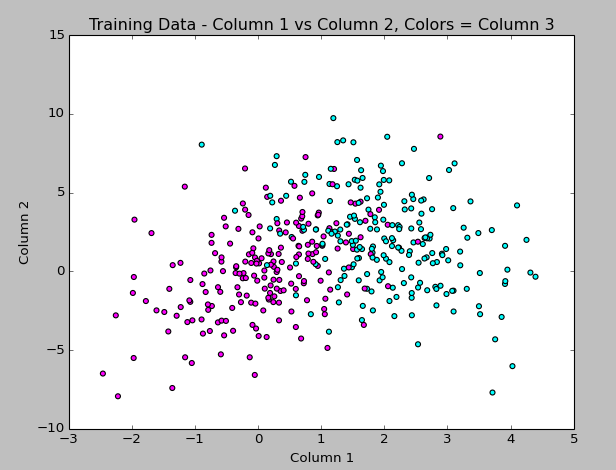
The code to generate this is:
#matplotlib, pyplot, numpy
import matplotlib.pyplot as plt
import numpy as np

#get data from training file
data = np.genfromtxt('train.txt', delimiter = ' ',
          dtype="float, float, int", names = "col1, col2, col3")

#set up color map
import matplotlib.colors as col
import matplotlib.cm as cm
my_colors = ["magenta","cyan"]
my_cmap = col.ListedColormap(my_colors[0:len(my_colors)], 'indexed')
cm.register_cmap(name="mycmap", cmap=my_cmap)

#plot column 1 vs 2 and use column 3 value to apply color
plt.scatter(data["col1"],data["col2"], c=data["col3"], cmap=cm.get_cmap("mycmap"))
plt.title("Training Data - Column 1 vs Column 2, Colors = Column 3")

#label axes and display
plt.xlabel("Column 1")
plt.ylabel("Column 2")
plt.show()
(Hey look at that… syntax highlighting via the Crayon plugin!)
I continued, and picked SciKit-Learn to do the automated Naive Bayes (I have to rewrite a function to do this myself for the project, but wanted to see how it should look). The classifying seemed to work without too much trouble, but colorizing the scatterplot points using matplotlib did not work the way I expected, so that part took the longest to figure out!
Here I plotted the results of the predicted boolean labels on the test data set based on the Naive Bayes model trained on the Train data set (both data sets provided by my professor). I know it’s not totally clear what I’m doing here, but the image shows the training data in magenta and cyan, with the test data overlayed, colored yellow or green based on the predicted class. I figure it’s a good sign that they overlap like this!
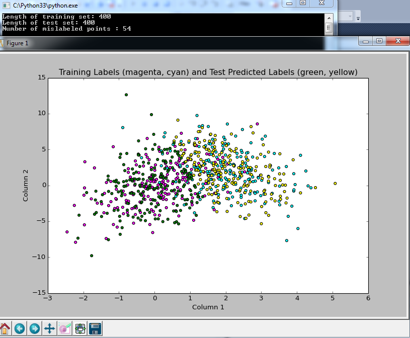
and here is the code:
#example from: http://scikit-learn.org/stable/modules/naive_bayes.html
#from sklearn import datasets
#iris = datasets.load_iris()
#from sklearn.naive_bayes import GaussianNB
#gnb = GaussianNB()
#y_pred = gnb.fit(iris.data, iris.target).predict(iris.data)
#print("Number of mislabeled points : %d" % (iris.target != y_pred).sum())

import numpy as np

#bring in data from files
ftrain = open("train.txt")
ftest = open("test.txt")
data_train = np.loadtxt(ftrain)
data_test = np.loadtxt(ftest)
#can't define 3rd column as integer, or it will collapse to 1D array and next line won't work?
Xtrn = data_train[:, 0:2]  # first 2 columns of training set
Ytrn = data_train[:, 2]  # last column, 1/0 labels
Xtst = data_test[:, 0:2]  # first 2 columns of test set
Ytst = data_test[:, 2]  # last column, 1/0 labels
print("Length of training set: %d " % len(Xtrn))
print("Length of test set: %d " % len(Xtst))

#NAIVE BAYES WITH SCIKIT LEARN
from sklearn.naive_bayes import GaussianNB
gnb = GaussianNB()
#array of predicted labels for test set based on training set?
y_prediction = gnb.fit(Xtrn, Ytrn).predict(Xtst)
#print(y_prediction)
GaussianNB()
print("Number of mislabeled points : %d" % (Ytst != y_prediction).sum())

import matplotlib.pyplot as plt

#set up colors
import matplotlib.colors as col
import matplotlib.cm as cm
my_colors = ["magenta","cyan","green","yellow"]
my_cmap = col.ListedColormap(my_colors[0:len(my_colors)], 'indexed')
#had to add these bounds and mynorm in order to use color indexes below the way I expected it to work
bounds=[0,1,2,3,4]
my_norm = col.BoundaryNorm(bounds, my_cmap.N)
#register the color map with name mycmap
cm.register_cmap(name="mycmap", cmap=my_cmap)

#converting 3rd column to int to use as color index in scatterplot
import array
data_color = array.array('i')
for yitem in data_train[:, 2]:
    data_color.append(int(yitem))
#bring in test data in to view it, adding 2 to the labels get the 3rd and 4th colors from the map
data2_color = array.array('i')
for yitem in y_prediction:
    data2_color.append(int(yitem + 2))

#plot column 1 vs 2 and use 3 to apply color
plt.scatter(data_train[:, 0],data_train[:, 1], c=data_color, cmap=cm.get_cmap("mycmap"), norm=my_norm)
plt.title("Training Labels (magenta, cyan) and Test Predicted Labels (green, yellow)")
#plot column 1 and 2 in test data with different colors based on prediction
plt.scatter(data_test[:, 0],data_test[:, 1], c=data2_color, cmap=cm.get_cmap("mycmap"), norm=my_norm)
#plt.colorbar()
plt.xlabel("Column 1")
plt.ylabel("Column 2")
plt.show()
The output from the classifier says that only 54 data points (out of 400) were not classified properly, based on comparing the predicted label to the true label provided in the test file. Sounds good to me!
So at this point, I’ve only just started the project, but I’m getting more used to Python, and feel like I’m making some progress. I have homework for another class that I’ll probably spend most of tomorrow doing, but I’ll be back this week updating as I continue this project.
Again, I’m not soliciting any help at the moment since I want to do this project on my own if at all possible, but after I turn it in on Thursday, I’d love any advice you have about improving the approach!
]]>The class to date has been mostly “math review” (which is not a review at all for me) and doing homework problems that take 4 pages of work to solve, such as “Show that the Gamma distribution is appropriately normalized”. Needless to say, I’m terrified of the impending midterm I have to take in about a month.
But in the meantime, we just got assigned our first project, having to do with Bayesian Classification! It’s due in 2 weeks and I barely know Python (we can choose any language for this project, and Python is one I’ve been wanting to learn and eventually master since it seems to be used frequently for Data Science work), and barely understand the Bayes classifier, but I’m still excited since learning how to do tasks like this are why I signed up for the class.
Here’s the full description of the project:
Given a training data set and a testing data set (text files), design different classifiers based on the training data set and test the designed classifiers on the test data set.
1. Bayes Classifier: Assume a Gaussian distribution for each class using maximum likelihood to estimate the conditional distribution P(x|ci) and p(ci). Then use Bayes Theory to compute the posterior probability.
2. Naive Bayes Classifier: Assume Gaussian Distribution for each class and assume conditional independence for each variable. Use maximum likelihood to estimate parameters and design a classifier.
3. Use nonparametric method, kernel method, to estimate p(x|ci), use maximum likelihood to estimate p(ci), and design a Bayes Classifier. Determine a suitable value for “h”.
4. Use K-Nearest-Neighbor method to classify the testing data using different k values.
5. Compare your results.
I think this is a lot to do in 2 weeks, especially since we have another difficult homework due in 1 week in this class, and I have homework for another class as well, but I’m going for it!
I had already installed Python into Visual Studio (which I already use for .NET development), and last night I installed scipy, mathplotlib, and numpy along with all of their dependencies. We’re not allowed to use pre-built functions and have to write our own classifiers, but I figure it can’t hurt to have a plan to check all of my work with something established!
My first triumph was importing the data from a text file, discovering it contained 3 columns of data, and creating this 3D plot last night:
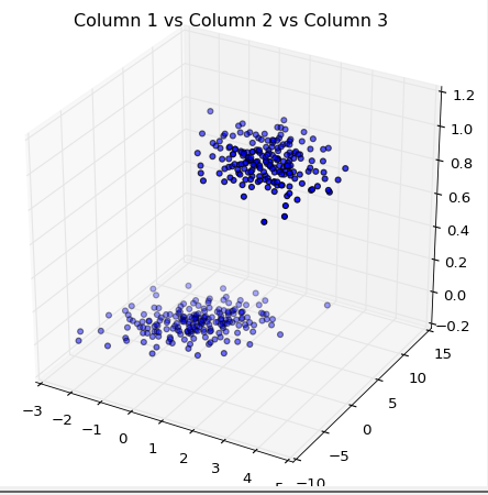
Here’s the code for my first-ever scatterplot in three dimensions:
import matplotlib.pyplot as plt
import numpy as np#get data from training file
data = np.genfromtxt(‘train.txt’, delimiter = ‘ ‘,
dtype=”float, float, float”, names = “col1, col2, col3”)#plot columns 1,2,3 as 3d scatterplot
from mpl_toolkits.mplot3d import Axes3D
import pylab
fig = pylab.figure()
ax = Axes3D(fig)
ax.scatter(data[“col1”],data[“col2”],data[“col3”],zdir=’z’)
plt.title(“Column 1 vs Column 2 vs Column 3”)
plt.show()
(note to self, get a syntax-highlighting wordpress plugin!)
Don’t tell me how to do any of this, since I don’t want to cheat! I’ll post my progress as I go along (though I won’t be back to working on this for about a week since the other homework is due first). Once I’m done with it, I’ll ask for feedback from those of you that know how I could have done it better, so I can keep learning.
I’m excited, and feeling time-crunched!
]]>